Thursday, September 10, 2020

Learning linear regression

The answers for the exercise in the previous post are 81,73,84. Now

In the previous post we discussed how predictions are obtained from linear regression when both the weights and the input features are known. So we are given the inputs and the weight, and we can produce the predicted output.

When we are given the inputs and the outputs for a number of items, we can find the weights such that the predicted output matches the actual output as well as possible. This is the task solved by machine learning.

Example

Continuing the shopping analogy, suppose we were given the contents of a number of shopping baskets and the total bill for each of them, and we were asked to figure out the price of each of the products (potatoes, carrots, and so on). From one basket, say 1kg of sirloin steak, 2kg of carrots, and a bottle of Chianti, even if we knew that the total bill is 35€, we couldn't determine the prices because there are many sets of prices that will yield the same total bill. With many baskets, however, we will usually be able to solve the problem.

But the problem is made harder by the fact that in the real world, the actual output isn’t always fully determined by the input, because of various factors that introduce uncertainty or “noise” into the process. You can think of shopping at a bazaar where the prices for any given product may vary from time to time, or a restaurant where the final damage includes a variable amount of tip. In such situations, we can estimate the prices but only with some limited accuracy.

Finding the weights that optimize the match between the predicted and the actual outputs in the training data is a classical statistical problem dating back to the 1800s, and it can be easily solved even for massive data sets.

Visualizing linear regression

A good way to get a feel for what linear regression can tell us is to draw a chart containing our data and our regression results. As a simple toy example our data set has one variable, the number of cups of coffee an employee drinks per day, and the number of lines of code written per day by that employee as the output. This is not a real data set as obviously there are other factors having an effect on the productivity of an employee other than coffee that interact in complex ways. The increase in productivity by increasing the amount of coffee will also hold only to a certain point after which the jitters distract too much.


When we present our data in the chart above as points where one point represents one employee, we can see that there is obviously a trend that drinking more coffee results in more lines of code being written (recall that this is completely made-up data). From this data set we can learn the coefficient, or the weight, related to coffee consumption, and by eye we can already say that it seems to be somewhere close to five, since for each cup of coffee consumed the number of lines programmed seems to go up roughly by five. For example, employees who drink around two cups of coffee per day seem to produce around 20 lines of code per day, and similarly at four cups of coffee, the amount of lines produced is around 30.

It can also be noted that employees who do not drink coffee at all also produce code, and is shown by the graph to be about ten lines. This number is the intercept term that we mentioned earlier. The intercept is another parameter in the model just like the weights are, that can be learned from the data. Just as in the life expectancy example it can be thought of as the starting point of our calculations before we have added in the effects of the input variable, or variables if we have more than one, be it coffee cups in this example, or cigarettes and vegetables in the previous one.

The line in the chart represents our predicted outcome, where we have estimated the intercept and the coefficient by using an actual linear regression technique called least squares. This line can be used to predict the number of lines produced when the input is the number of cups of coffee. Note that we can obtain a prediction even if we allow only partial cups (like half, 1/4 cups, and so on).

Let's study the link between the total number of years spent in school (including everything between preschool and university) and life expectancy. Here is data from three different countries displayed in a figure represented by dots:

We have one country where the average number of years in school is 10 and life expectancy is 57 years, another country where the average number of years in school is 13 and life expectancy is 53 years, and a third country where the average number of years in school is 20 and life expectancy is 80 years.

You can drag the end points of the solid line to position the line in such a way that it follows the trend of the data points. Note that you will not be able to get the line fit perfectly with the data points, and this is fine: some of the data points will lie above the line, and some below it. The most important part is that the line describes the overall trend.

After you have positioned the line you can use it to predict the life expectancy.

Given the data, what can you tell about the life expectancy of people who have 15 years of education? Important: Notice that even if you can obtain a specific prediction, down to a fraction of a year, by adjusting the line, you may not necessarily be able to give a confident prediction. Take the limited amount of data into account when giving your answer.

It should be pointed out that studies like those used in the above exercises cannot identify causal relationships. In other words, from this data alone, it is impossible to say whether studying actually increases life expectancy through a better-informed and healthier life-style or other mechanisms, or whether the apparent association between life expectancy and education is due to underlying factors that affects both. It is likely that, for example, in countries where people tend to be highly educated, nutrition, healthcare, and safety are also better, which increases life expectancy. With this kind of simple analysis, we can only identify associations, which can nevertheless be useful for prediction.

Share:

Wednesday, September 9, 2020

Regression

The difference between classification and regression

There is a small but important difference in the kind of predictions that we should produce in different scenarios. While for example the nearest neighbor classifier chooses a class label for any item out of a given set of alternatives (like spam/ham, or 0,1,2,...,9), linear regression produces a numerical prediction that is not constrained to be an integer (a whole number as opposed to something like 3.14). So linear regression is better suited in situations where the output variable can be any number like the price of a product, the distance to an obstacle, the box-office revenue of the next Star Wars movie, and so on.

The basic idea in linear regression is to add up the effects of each of the feature variables to produce the predicted value. The technical term for the adding up process is linear combination. The idea is very straightforward, and it can be illustrated by your shopping bill.

Thinking of linear regression as a shopping bill

Suppose you go to the grocery store and buy 2.5 kg potatoes, 1.0 kg carrots, and two bottles of milk. If the price of potatoes is 2€ per kg, the price of carrots is 4€ per kg, and a bottle of milk costs 3€, then the bill, calculated by the cashier, totals 2.5 × 2€ + 1.0 × 4€ + 2 × 3€ = 15€. In linear regression, the amount of potatoes, carrots, and milk are the inputs in the data. The output is the cost of your shopping, which clearly depends on both the price and how much of each product you buy.

The word linear means that the increase in the output when one input feature is increased by some fixed amount is always the same. In other words, whenever you add, say, two kilos of carrots into your shopping basket, the bill goes up 8€. When you add another two kilos, the bill goes up another 8€, and if you add half as much, 1kg, the bill goes up exactly half as much, 4€.

Coefficients or weights

In linear regression terminology, the prices of the different products would be called coefficients or weights (this may appear confusing since we measured the amount of potatoes and carrots by weight, but not let yourself be tricked by this). One of the main advantages of linear regression is its easy interpretability: the learned weights may in fact be more interesting than the predictions of the outputs.

For example, when we use linear regression to predict the life expectancy, the weight of smoking (cigarettes per day) is about minus half a year, meaning that smoking one cigarette more per day takes you on the average half a year closer to termination. Likewise, the weight of vegetable consumption (handful of vegetables per day) has weight plus one year, so eating a handful of greens gives every day gives you on the average one more year.

Suppose that an extensive study is carried out, and it is found that in a particular country, the life expectancy (the average number of years that people live) among non-smoking women who don't eat any vegetables is 80 years. Suppose further that on the average, men live 5 years less. Also take the numbers mentioned above: every cigarette per day reduces the life expectancy by half a year, and a handful of veggies per day increases it by one year.

Calculate the life expectancies for the following example cases:

For example, the first case is a male (subtract 5 years), smokes 8 cigarettes per day (subtract 8 × 0.5 = 4 years), and eats two handfuls of veggies per day (add 2 × 1 = 2 years), so the predicted life expectancy is 80 - 5 - 4 + 2 = 73 years.

GenderSmoking (cigarettes per day)Vegetables (handfuls per day)Life expectancy (years)
male8273
male06A
female161B
female04C

Your task: Enter the correct value as an integer (whole number) for the missing sections A, B, and C above.

We'll see the answers in the next post.

Share:

Tuesday, September 8, 2020

Using nearest neighbors to predict user behavior

man and woman listening to music on the phone

A typical example of an application of the nearest neighbor method is predicting user behavior in AI applications such as recommendation systems.

The idea is to use the very simple principle that users with similar past behavior tend to have similar future behavior. Imagine a music recommendation system that collects data about users’ listening behavior. Let’s say you have listened to 1980s disco music (just for the sake of argument). One day, the service provider gets their hands on a hard-to-find 1980 disco classic, and adds it into the music library. The system now needs to predict whether you will like it or not. One way of doing this is to use information about the genre, the artist, and other metadata, entered by the good people of the service provider. However, this information is relatively scarce and coarse and it will only be able to give rough predictions.

What current recommendation systems use instead of the manually entered metadata, is something called collaborative filtering. The collaborative aspect of it is that it uses other users’ data to predict your preferences. The word “filter” refers to the fact that you will be only recommended content that passes through a filter: content that you are likely to enjoy will pass, other content will not (these kind of filters may lead to the so called filter bubbles.

Now let’s say that other users who have listened to 80s disco music enjoy the new release and keep listening to it again and again. The system will identify the similar past behavior that you and other 80s disco fanatics share, and since other users like you enjoy the new release, the system will predict that you will too. Hence it will show up at the top of your recommendation list. In an alternative reality, maybe the added song is not so great and other users with similar past behavior as yours don't really like it. In that case, the system wouldn't bother recommending it to you, or at least it wouldn't be at the top of the list of recommendations for you.

Let's build a simple recommendation system for an online shopping application where the users' purchase history is recorded and used to predict which products the user is likely to buy next.

We have data from six users. For each user, we have recorded their recent shopping history of four items and the item they bought after buying these four items:


UserShopping HistoryPurchase
Sanniboxing glovesMoby Dick (novel)headphonessunglassescoffee beans
Jounit-shirtcoffee beanscoffee makercoffee beanscoffee beans
Janinasunglassessneakerst-shirtsneakersragg wool socks
Henrik2001: A Space Odyssey (dvd)headphonest-shirtboxing glovesflip flops
Villet-shirtflip flopssunglassesMoby Dick (novel)sunscreen
TeemuMoby Dick (novel)coffee beans2001: A Space Odyssey (dvd)headphonescoffee beans

The most recent purchase is the one in the rightmost column, so for example, after buying a t-shirt, flip flops, sunglasses, and Moby Dick (novel), Ville bought sunscreen. Our hypothesis is that after buying similar items, other users are also likely to buy sunscreen.

To apply the nearest neighbor method, we need to define what we mean by nearest. This can be done in many different ways, some of which work better than others. Let’s use the shopping history to define the similarity (“nearness”) by counting how many of the items have been purchased by both users.

For example, users Ville and Henrik have both bought a t-shirt, so their similarity is 1. Note that flip flops doesn't count because we don't include the most recent purchase when calculating the similarity — it is reserved for another purpose.

Our task is to predict the next purchase of customer Travis who has bought the following products:


UserShopping HistoryPurchase
Travisgreen teat-shirtsunglassesflip flops?

You can think of Travis being our test data, and the above six users make our training data.

Proceed as follows:

  1. Calculate the similarity of Travis relative to the six users in the training data (done by adding together the number of similar purchases by the users).
  2. Having calculated the similarities, identify the user who is most similar to Travis by selecting the largest of the calculated similarities.
  3. Predict what Travis is likely to purchase next by looking at the most recent purchase (the rightmost column in the table) of the most similar user from the previous step.
When you calculate the similarities between Travis and all the other users, Ville and Travis will have the largest similarity with a similarity of 3. Since Ville's latest purchase was sunscreen, we will recommend it also to Travis.

In the above example, we only had six users’ data and our prediction was probably very unreliable. However, online shopping sites often have millions of users, and the amount of data they produce is massive. In many cases, there are a horde of users whose past behavior is very similar to yours, and whose purchase history gives a pretty good indication of your interests.

These predictions can also be self-fulfilling prophecies in the sense that you are more likely to buy a product if it is recommended to you by the system, which makes it tricky to evaluate how well they actually work. The same kind of recommendation systems are also used to recommend music, movies, news, and social media content to users. In the context of news and social media, filters created by such systems can lead to filter bubbles.

Share:

Monday, September 7, 2020

The nearest neighbor classifier


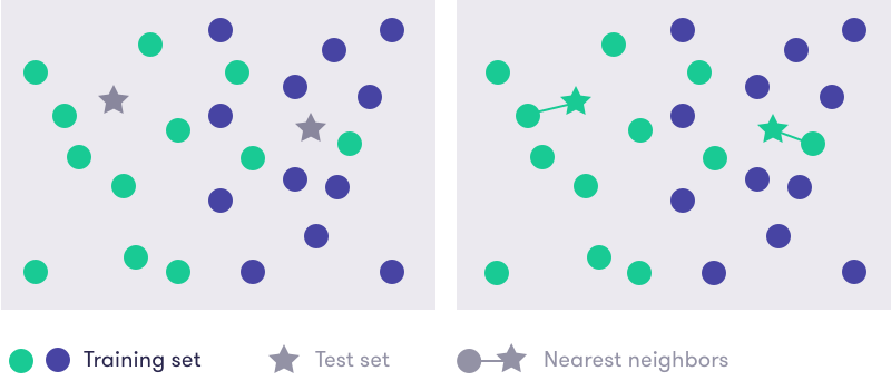
The nearest neighbor classifier is among the simplest possible classifiers. When given an item to classify, it finds the training data item that is most similar to the new item, and outputs its label. An example is given in the following diagram. 


nearest neighbor classifier 

 In the above diagram, we show a collection of training data items, some of which belong to one class (green) and other to another class (blue). In addition, there are two test data items, the stars, which we are going to classify using the nearest neighbor method.


The two test items are both classified in the “green” class because their nearest neighbors are both green (see diagram (b) above).

The position of the points in the plot represents in some way the properties of the items. Since we draw the diagram on a flat two-dimensional surface – you can move in two independent directions: up-down or left-right – the items have two properties that we can use for comparison. Imagine for example representing patients at a clinic in terms of their age and blood-sugar level. But the above diagram should be taken just as a visual tool to illustrate the general idea, which is to relate the class values to similarity or proximity (nearness). The general idea is by no means restricted to two dimensions and the nearest neighbor classifier can easily be applied to items that are characterized by many more properties than two. 

What do we mean by nearest?

An interesting question related to (among other things) the nearest neighbor classifier is the definition of distance or similarity between instances. In the illustration above, we tacitly assumed that the standard geometric distance, technically called the Euclidean distance, is used. This simply means that if the points are drawn on a piece of paper (or displayed on your screen), you can measure the distance between any two items by pulling a piece of thread straight from one to the other and measuring the length.

In the MNIST digit recognition case, one common way to measure image similarity is to count pixel-by-pixel matches. In other words, we compare the pixels in the top-left corner of each image to one another and if the more similar color (shade of gray) they are, the more similar the two images are. We also compare the pixels in the bottom-right corner of each image, and all pixels inbetween. This technique is quite sensitive to shifting or scaling the images: if we take an image of a '1' and shift it ever so slightly either left or right, the outcome is that the two images (before and after the shift) are very different because the black pixels are in different positions in the two images. Fortunately, the MNIST data has been preprocessed by centering the images so that this problem is alleviated.

Defining ‘nearest’

Using the geometric distance to decide which is the nearest item may not always be reasonable or even possible: the type of the input may, for example, be text, where it is not clear how the items are drawn in a geometric representation and how distances should be measured. You should therefore choose the distance metric on a case-by-case basis.


Share:

Sunday, September 6, 2020

Learning without a teacher: unsupervised learning

AI Academy: What is Machine Learning?

In the previous post we discussed supervised learning where the correct answers are available, and the task of the machine learning algorithm is to find a model that predicts them based on the input data.

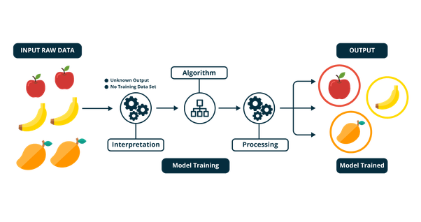
In unsupervised learning, the correct answers are not provided. This makes the situation quite different since we can't build the model by making it fit the correct answers on training data. It also makes the evaluation of performance more complicated since we can't check whether the learned model is doing well or not.

Typical unsupervised learning methods attempt to learn some kind of “structure” underlying the data. This can mean, for example, visualization where similar items are placed near each other and dissimilar items further away from each other. It can also mean clustering where we use the data to identify groups or “clusters” of items that are similar to each other but dissimilar from data in other clusters.

Example

As a concrete example, grocery store chains collect data about their customers' shopping behavior (that's why you have all those loyalty cards). To better understand their customers, the store can either visualize the data using a graph where each customer is represented by a dot and customers who tend to buy the same products are placed nearer each other than customers who buy different products. Or, the store could apply clustering to obtain a set of customer groups such as ‘low-budget health food enthusiasts’, ‘high-end fish lovers’, ‘soda and pizza 6 days a week’, and so on. Note that the machine learning method would only group the customers into clusters, but it wouldn't automatically generate the cluster labels (‘fish lovers’ and so on). This task would be left for the user.

Yet another example of unsupervised learning can be termed generative modeling. This has become a prominent approach since the last few years as a deep learning technique called generative adversarial networks (GANs) has lead to great advances. Given some data, for example, photographs of people's faces, a generative model can generate more of the same: more real-looking but artificial images of people's faces.

Share:

Saturday, September 5, 2020

Humans teaching machines: supervised learning

Supervised Machine learning - Javatpoint

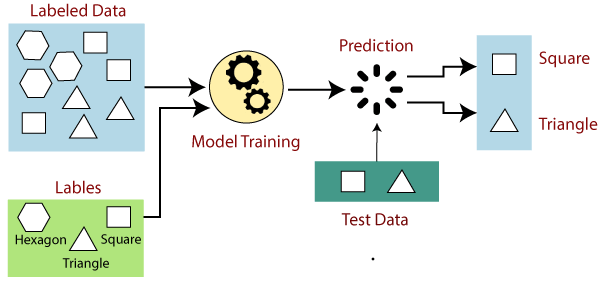
Instead of manually writing down exact rules to do the classification, the point in supervised machine learning is to take a number of examples, label each one by the correct label, and use them to “train” an AI method to automatically recognize the correct label for the training examples as well as (at least hopefully) any other images. This of course requires that the correct labels are provided, which is why we talk about supervised learning. The user who provides the correct labels is a supervisor who guides the learning algorithm towards correct answers so that eventually, the algorithm can independently produce them.

In addition to learning how to predict the correct label in a classification problem, supervised learning can also be used in situations where the predicted outcome is a number. Examples include predicting the number of people who will click a Google ad based on the ad content and data about the user’s prior online behavior, predicting the number of traffic accidents based on road conditions and speed limit, or predicting the selling price of real estate based on its location, size, and condition. These problems are called regression. You probably recognize the term linear regression, which is a classical, still very popular technique for regression.

Example

Suppose we have a data set consisting of apartment sales data. For each purchase, we would obviously have the price that was paid, together with the size of the apartment in square meters (or square feet, if you like), and the number of bedrooms, the year of construction, the condition (on a scale from “disaster“ to “spick and span”). We could then use machine learning to train a regression model that predicts the selling price based on these features.

There are a couple potential mistakes that I'd like to make you aware of. They are related to the fact that unless you are careful with the way you apply machine learning methods, you could become too confident about the accuracy of your predictions, and be heavily disappointed when the accuracy turns out to be worse than expected.

The first thing to keep in mind in order to avoid big mistakes, is to split your data set into two parts: the training data and the test data. We first train the algorithm using only the training data. This gives us a model or a rule that predicts the output based on the input variables.

To assess how well we can actually predict the outputs, we can't count on the training data. While a model may be a very good predictor in the training data, it is no proof that it can generalize to any other data. This is where the test data comes in handy: we can apply the trained model to predict the outputs for the test data and compare the predictions to the actual outputs (for example, future apartment sale prices).

Too fit to be true! Overfitting alert

It is very important to keep in mind that the accuracy of a predictor learned by machine learning can be quite different in the training data and in separate test data. This is the so-called overfitting phenomenon, and a lot of machine learning research is focused on avoiding it one way or another. Intuitively, overfitting means trying to be too smart. When predicting the success of a new song by a known artist, you can look at the track record of the artist's earlier songs, and come up with a rule like “if the song is about love, and includes a catchy chorus, it will be top-20”. However, maybe there are two love songs with catchy choruses that didn't make the top-20, so you decide to continue the rule “...except if Sweden or yoga are mentioned” to improve your rule. This could make your rule fit the past data perfectly, but it could in fact make it work worse on future test data.

Machine learning methods are especially prone to overfitting because they can try a huge number of different “rules” until one that fits the training data perfectly is found. Especially methods that are very flexible and can adapt to almost any pattern in the data can overfit unless the amount of data is enormous. For example, compared to quite restricted linear models obtained by linear regression, neural networks can require massive amounts of data before they produce reliable prediction.

Learning to avoid overfitting and choose a model that is not too restricted, nor too flexible, is one of the most essential skills of a data scientist.

In the next post we'll discuss about unsupervised learning.

Share:

Friday, September 4, 2020

MNIST dataset

MNIST Reborn, Restored and Expanded: Additional 50K Training Samples | by  Synced | SyncedReview | Medium

Every machine learning student knows about the MNIST dataset. Fewer know what the acronym stands for. In fact, we had to look it up to be able to tell you that the M stands for Modified, and NIST stands for National Institute of Standards and Technology. Now you probably know something that an average machine learning expert doesn’t!

Handwritten digits are a classic case that is often used when discussing why we use machine learning, and we will make no exception.

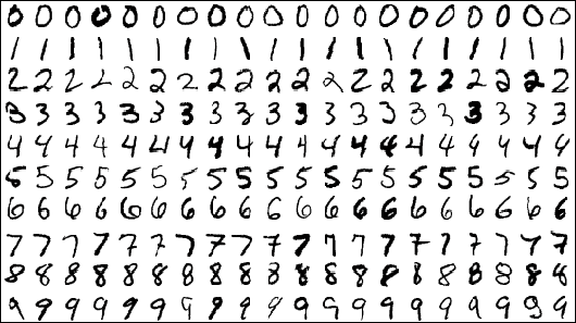
Below you can see examples of handwritten images from the very commonly used MNIST dataset.


The correct label (what digit the writer was supposed to write) is shown above each image. Note that some of the "correct” class labels are questionable: see for example the second image from left: is that really a 7, or actually a 4?

In the most common machine learning problems, exactly one class value is correct at a time. This is also true in the MNIST case, although as we said, the correct answer may often be hard to tell. In this kind of problem, it is not possible that an instance belongs to multiple classes (or none at all) at the same time. What we would like to achieve is an AI method that can be given an image like the ones above, and automatically spits out the correct label (a number between 0 and 9).

The roots of machine learning are in statistics, which can also be thought of as the art of extracting knowledge from data. Especially methods such as linear regression and Bayesian statistics, which are both already more than two centuries old (!), are even today at the heart of machine learning.

The area of machine learning is often divided in subareas according to the kinds of problems being attacked. A rough categorization is as follows:

Supervised learning: We are given an input, for example a photograph with a traffic sign, and the task is to predict the correct output or label, for example which traffic sign is in the picture (speed limit, stop sign, etc.). In the simplest cases, the answers are in the form of yes/no (we call these binary classification problems).

Unsupervised learning: There are no labels or correct outputs. The task is to discover the structure of the data: for example, grouping similar items to form “clusters”, or reducing the data to a small number of important “dimensions”. Data visualization can also be considered unsupervised learning.

Reinforcement learning: Commonly used in situations where an AI agent like a self-driving car must operate in an environment and where feedback about good or bad choices is available with some delay. Also used in games where the outcome may be decided only at the end of the game.

The categories are somewhat overlapping and fuzzy, so a particular method can sometimes be hard to place in one category. For example, as the name suggests, so-called semisupervised learning is partly supervised and partly unsupervised.

When it comes to machine learning, we will focus primarily on supervised learning, and in particular, classification tasks. In classification, we observe in input, such as a photograph of a traffic sign, and try to infer its “class”, such as the type of sign (speed limit 80 km/h, pedestrian crossing, stop sign, etc.). Other examples of classification tasks include: identification of fake Twitter accounts (input includes the list of followers, and the rate at which they have started following the account, and the class is either fake or real account) and handwritten digit recognition (input is an image, class is 0,...,9).

We shall continue our discuss in the next post which will focus on supervised learning.

Share:

Thursday, September 3, 2020

Naive Bayes classification

Naive Bayesian

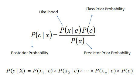
One of the most useful applications of the Bayes rule is the so-called naive Bayes classifier.

The Bayes classifier is a machine learning technique that can be used to classify objects such as text documents into two or more classes. The classifier is trained by analyzing a set of training data, for which the correct classes are given.

The naive Bayes classifier can be used to determine the probabilities of the classes given a number of different observations. The assumption in the model is that the feature variables are conditionally independent given the class (we will not discuss the meaning of conditional independence in this course. For our purposes, it is enough to be able to exploit conditional independence in building the classifier).

Why we call it “naive”

Using spam filters as an example, the idea is to think of the words as being produced by choosing one word after the other so that the choice of the word depends only on whether the message is spam or ham. This is a crude simplification of the process because it means that there is no dependency between adjacent words, and the order of the words has no significance. This is in fact why the method is called naive.

Real world application: spam filters

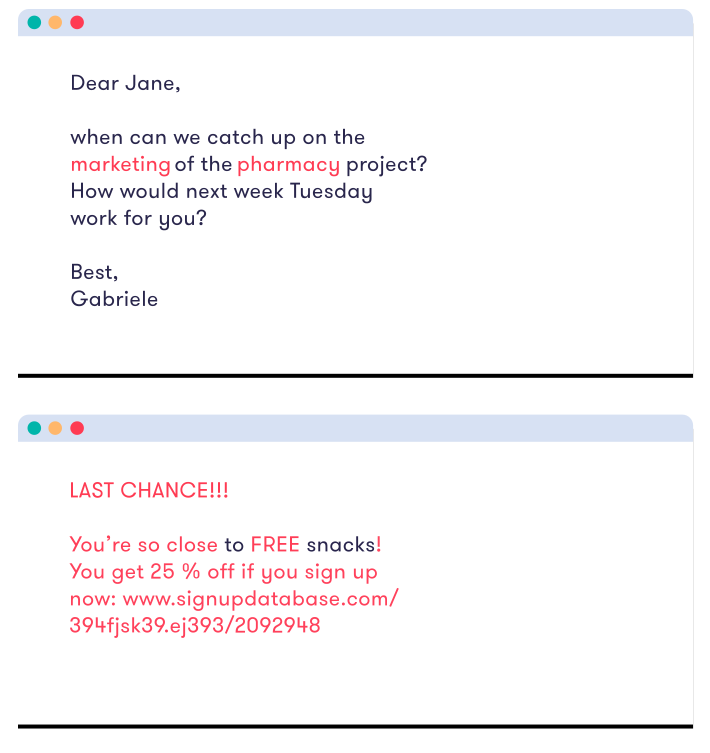
We will use a spam email filter as a running example for illustrating the idea of the naive Bayes classifier. Thus, the class variable indicates whether a message is spam (or “junk email”) or whether it is a legitimate message (also called “ham”). The words in the message correspond to the feature variables, so that the number of feature variables in the model is determined by the length of the message.

Because the model is based on the idea that the words can be processed independently, we can identify specific words that are indicative of either spam ("FREE", "LAST") or ham ("meeting", "algorithm").

a normal email and a spam email

Despite its naivete, the naive Bayes method tends to work very well in practice. This is a good example of the common saying in statistics, “all models are wrong, but some are useful” means (the aphorism is generally attributed to statistician George E.P. Box).

Estimating parameters

To get started, we need to specify the prior odds for spam (against ham). For simplicity assume this to be 1:1 which means that on the average half of the incoming messages are spam (in reality, the amount of spam is probably much higher).

To get our likelihood ratios, we need two different probabilities for any word occurring: one in spam messages and another one in ham messages.

The word distributions for the two classes are best estimated from actual training data that contains some spam messages as well as legitimate messages. The simplest way is to count how many times each word, abacus, acacia, ..., zurg, appears in the data and divide the number by the total word count.

To illustrate the idea, let’s assume that we have at our disposal some spam and some ham. You can easily obtain such data by saving a batch of your emails in two files.

Assume that we have calculated the number of occurrences of the following words (along with all other words) in the two classes of messages:


wordspamham
million15698
dollars29119
adclick510
conferences012
total95791306438

We can now estimate that the probability that a word in a spam message is million, for example, is about 156 out of 95791, which is roughly the same as 1 in 614. Likewise, we get the estimate that 98 out of 306438 words, which is about the same as 1 in 3127, in a ham message are million. Both of these probability estimates are small, less than 1 in 500, but more importantly, the former is higher than the latter: 1 in 614 is higher than 1 in 3127. This means that the likelihood ratio, which is the first ratio divided by the second ratio, is more than one. To be more precise, the ratio is (1/614) / (1/3127) = 3127/614 = 5.1 (rounded to one decimal digit).

Zero means trouble

One problem with estimating the probabilities directly from the counts is that zero counts lead to zero estimates. This can be quite harmful for the performance of the classifier – it easily leads to situations where the posterior odds are 0/0, which is nonsense. The simplest solution is to use a small lower bound for all probability estimates. The value 1/100000, for instance, does the job.

Using the above logic, we can determine the likelihood ratio for all possible words without having to use zero, giving us the following likelihood ratios:

wordlikelihood ratio
million5.1
dollars0.8
adclick53.2
conferences0.3
We are now ready to apply the method to classify new messages.

Example: is it spam or ham?

Once we have the prior odds and the likelihood ratios calculated, we are ready to apply the Bayes rule, which we already practiced in the medical diagnosis case as our example. The reasoning goes just like it did before: we update the odds of spam by multiplying it by the likelihood ratio. To remind ourselves of the procedure, let's try a message with a single word to begin with. For the prior odds, as agreed above, you should use odds 1:1.
Share:

Wednesday, September 2, 2020

The Bayes rule

Bayes' rule with a simple and practical example | by Tirthajyoti Sarkar |  Towards Data Science

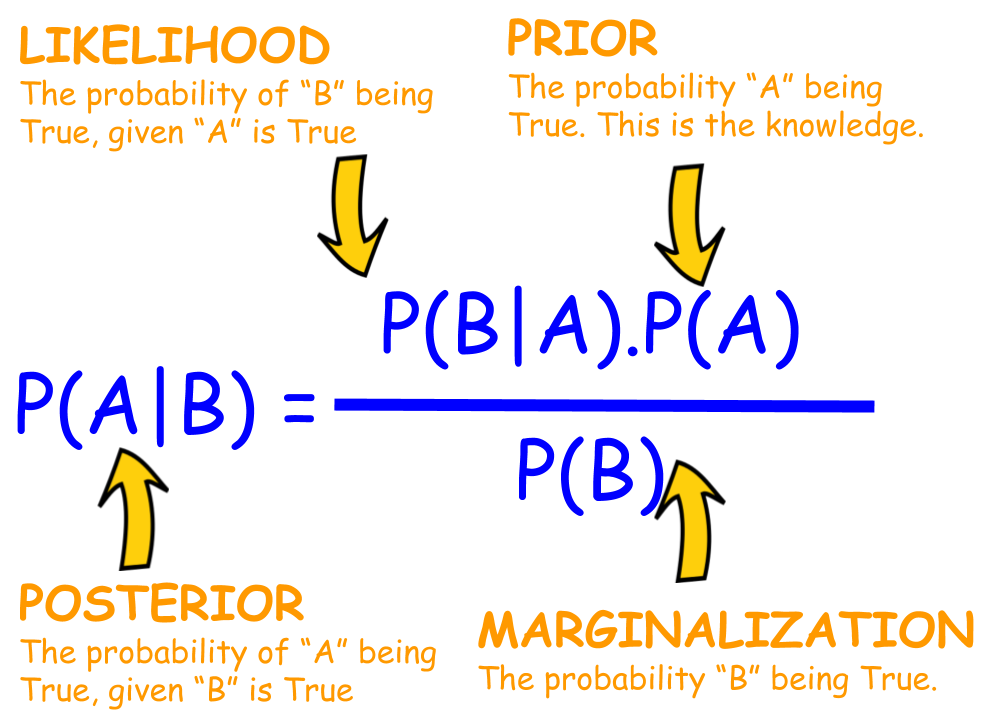
Now we will discuss one very important formula which can be used to weigh conflicting pieces of evidence in medicine, in a court of law, and in many (if not all) scientific disciplines.The formula is called the Bayes rule (or the Bayes formula). 

We will start by demonstrating the power of the Bayes rule by means of a simple medical diagnosis problem where it highlights how poorly our intuition is suited for combining conflicting evidence. We will then show how the Bayes rule can be used to build AI methods that can cope with conflicting and noisy observations.

Prior and posterior odds

The Bayes rule can be expressed in many forms. The simplest one is in terms of odds. The idea is to take the odds for something happening (against it not happening), which we´ll call prior odds. The word prior refers to our assessment of the odds before obtaining some new information that may be relevant. The purpose of the formula is to update the prior odds when new information becomes available, to obtain the posterior odds, or the odds after obtaining the information (the dictionary meaning of posterior is “something that comes after, later.)”

How odds change

In order to weigh the new information, and decide how the odds change when it becomes available, we need to consider how likely we would be to encounter this information in alternative situations. Let’s take as an example, the odds that it will rain later today. Imagine getting up in the morning in Finland. The chances of rain are 206 in 365 (including rain, snow, and hail. Brrr). The number of days without rain is therefore 159. This converts to prior odds of 206:159 for rain, so the cards are stacked against you already before you open your eyes.

However, after opening your eyes and taking a look outside, you notice it’s cloudy. Suppose the chances of having a cloudy morning on a rainy day are 9 out of 10 – that means that only one out of 10 rainy days start out with blue skies. But sometimes there are also clouds without rain: the chances of having clouds on a rainless day are 1 in 10. Now how much higher are the chances of clouds on a rainy day compared to a rainless day? Think about this carefully as it will be important to be able to comprehend the question and obtain the answer in what follows.

The answer is that the chances of clouds are nine times higher on a rainy day than on a rainless day: on a rainy day the chances are 9 out of 10, whereas on a rainless day the chances of clouds are 1 out of 10, and that makes nine times higher.

Note that even thought the two probabilities 9/10 and 1/10 sum up to 9/10 + 1/10 = 1, this is by no means always the case. In some other town, the mornings of rainy days could be cloudy eight times out of ten. This, however, would not mean that the rainless days are cloudy two times out of ten. You'll have to be careful to get the calculations right. (But never mind if you make a mistake or two – don't give up! The Bayes rule is a fundamental thinking tool for everyone of us.)

Likelihood ratio

The above ratio (nine times higher chance of clouds on a rainy day than on a rainless day) is called the likelihood ratio. More generally, the likelihood ratio is the probability of the observation in case the event of interest (in the above, rain), divided by the probability of the observation in case of no event (in the above, no rain). Please read the previous sentence a few times. It may look a little intimidating, but it´s not impossible to digest if you just focus carefully. We will walk you through the steps in detail, just don´t lose your nerve. We´re almost there.

So we concluded that on a cloudy morning, we have: likelihood ratio = (9/10) / (1/10) = 9

The mighty Bayes rule for converting prior odds into posterior odds is – ta-daa! – as follows: posterior odds = likelihood ratio × prior odds

Now you are probably thinking: Hold on, that’s the formula? It’s a frigging multiplication! That is the formula – we said it’s simple, didn’t we? You wouldn’t imagine that a simple multiplication can be used for all kinds of incredibly useful applications, but it can. We’ll study a couple examples which will demonstrate this.

The Bayes rule in practice: breast cancer screening

Our first realistic application is a classical example of using the Bayes rule, namely medical diagnosis. This example also illustrates a common bias in dealing with uncertain information called the base-rate fallacy.

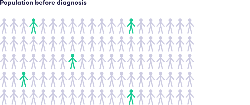
image illustrating false positives and negatives for cancer screening


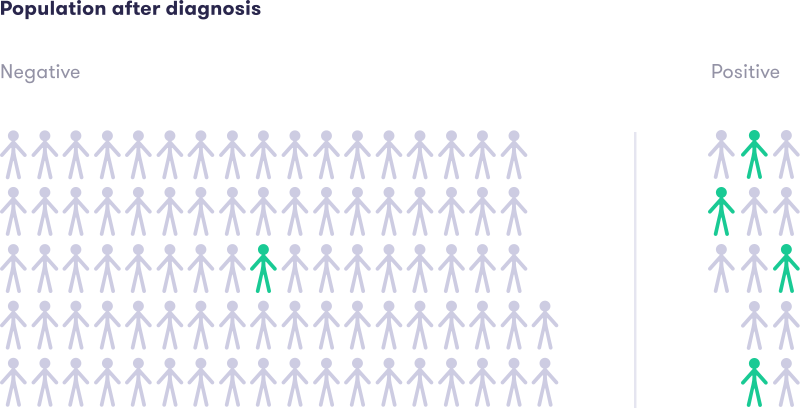
image illustrating false positives and negatives for cancer screening

Consider mammographic screening for breast cancer. Using made up percentages for the sake of simplifying the numbers, let’s assume that 5 in 100 women have breast cancer. Suppose that if a person has breast cancer, then the mammograph test will find it 80 times out of 100. When the test comes out suggesting that breast cancer is present, we say that the result is positive, although of course there is nothing positive about this for the person being tested (a technical way of saying this is that the sensitivity of the test is 80%).

The test may also fail in the other direction, namely to indicate breast cancer when none exists. This is called a false positive finding. Suppose that if the person being tested actually doesn’t have breast cancer, the chances that the test nevertheless comes out positive are 10 in 100. (In technical terms, we would say that the specificity of the test is 90%.)

Based on the above probabilities, you are able to calculate the likelihood ratio. You'll find use for it in the next exercise. If you forgot how the likelihood ratio is calculated, you may wish to check the terminology box earlier in this section and revisit the rain example.


Note: You can use the above diagram with stick figures to validate that your result is in the ballpark (about right) but note that diagram isn't quite precise. Out of the 95 women who don't have cancer (the gray figures in the top panel), about nine and a half are expected to get a (false) positive result. The remaining 84 and a half are expected to get a (true) negative result. We didn't want to be so cruel as to cut people – even stick figures – in half, so we used 10 and 85 as an approximation.

Share:

Tuesday, September 1, 2020

Odds and probability

 Instead of perfect information, there is a host of unknown possibilities, ranging from missing information to deliberate deception.

Take a self-driving car for example — you can set the goal to get from A to B in an efficient and safe manner that follows all laws. But what happens if the traffic gets worse than expected, maybe because of an accident ahead? Sudden bad weather? Random events like a ball bouncing in the street, or a piece of trash flying straight into the car’s camera?

self driving car at stop sign

A self-driving car needs to use a variety of sensors, including sonar-like ones and cameras, to detect where it is and what is around it. These sensors are never perfect as the data from the sensors always includes some errors and inaccuracies called “noise”. It is very common then that one sensor indicates that the road ahead turns left, but another sensor indicates the opposite direction. This needs to be resolved without always stopping the car in case of even a slightest amount of noise.

Probability

One of the reasons why modern AI methods actually work in real-world problems – as opposed to most of the earlier “good old-fashioned" methods in the 1960-1980s – is their ability to deal with uncertainty.

The history of AI has seen various competing paradigms for handling uncertain and imprecise information. For example, you may have heard of fuzzy logic. Fuzzy logic was for a while a contender for the best approach to handle uncertain and imprecise information and used in many customer-applications such as washing machines where the machine could detect the dirtiness (a matter of degrees, not only dirty or clean) and adjust the program accordingly.

However, probability has turned out to be the best approach for reasoning under uncertainty, and almost all current AI applications are based, to at least some degree, on probabilities.

hand holding playing cards

Why probability matters

We are perhaps most familiar with applications of probability in games: what are the chances of getting three of a kind in poker (about 1 in 47), what are the chances of winning in the lottery (very small), and so on. However, far more importantly, probability can also be used to quantify and compare risks in everyday life: what are the chances of crashing your car if you exceed the speed limit, what are the chances that the interest rates on your mortgage will go up by five percentage points within the next five years, or what are the chances that AI will automate particular tasks such as detecting fractured bones in X-ray images or waiting tables in a restaurant.

The most important lesson about probability that we’d like you to take away is not probability calculus. Instead, it is the ability to think of uncertainty as a thing that can be quantified at least in principle. This means that we can talk about uncertainty as if it were a number: numbers can be compared (“is this thing more probable than that thing”), and they can often be measured.

Granted, measuring probabilities is hard: we usually need many observations about a phenomenon to draw conclusions. However, by systematically collecting data, we can critically evaluate probabilistic statements, and our numbers can sometimes be found to be right or wrong. In other words, the key lesson is that uncertainty is not beyond the scope of rational thinking and discussion, and probability provides a systematic way of doing just that.

The fact that uncertainty can be quantified is of paramount importance, for example, in decisions concerning vaccination or other public policies. Before entering the market, any vaccine is clinically tested, so that its benefits and risks have been quantified. The risks are never known to the minutest detail, but their magnitude is usually known to sufficient degree that it can be argued whether the benefits outweigh the risks.

If we think of uncertainty as something that can’t be quantified or measured, the uncertainty aspect may become an obstacle for rational discussion. We may for example argue that since we don’t know exactly whether a vaccine may cause a harmful side-effect, it is too dangerous to use. However, this may lead us to ignore a life-threatening disease that the vaccine will eradicate. In most cases, the benefits and risks are known to sufficient precision to clearly see that one is more significant than the other. 

The discussion above is useful in many everyday scenarios and professionally: for example, medical doctors, judges in a court of law, or investors have to process uncertain information and make rational decisions based on them. Since this is an AI course, we will discuss how probability can be used to automate uncertain reasoning. The examples we will use include medical diagnosis (although it is usually not a task that we’d wish to fully automate), and identifying fraudulent email messages (“spam”).

Odds

Probably the easiest way to represent uncertainty is through odds. They make it particularly easy to update beliefs when more information becomes available (we will return to this in the next section).

Before we proceed any further, we should make sure you are comfortable with doing basic manipulations on ratios (or fractions). As you probably recall, fractions are numbers like 3/4 or 21/365. We will need to multiply and divide such things, so it's good to refresh these operations if you feel unsure about them. A compact presentation for those who just need a quick reminder is Wikibooks: Multiplying Fractions. Another fun animated presentation of the basic operations is Math is Fun: Using Rational Numbers. Feel free to consult your favorite source if necessary.

By odds, we mean an expression like 3:1 (three to one), which means that we expect that for every three cases of an outcome, for example winning a bet, there is one case of the opposite outcome, not winning the bet. (In gambling terms, the odds are usually given from the bookmakers point of view, so 3:1 usually means that your chances of winning are 1:3.) The other way to express the same would be to say that the chances of winning are 3/4 (three in four). These are called natural frequencies since they involve only whole numbers. With whole numbers, it is easy to imagine, for example, four people out of whom, three have brown eyes. Or four days out of which it rains on three (if you’re in Helsinki).

three people with brown eyes, one person with blue eyes

Why we use odds and not percentages

Three out of four is of course the same as 75% (mathematicians prefer to use fractions like 0.75 instead of percentages). It has been found that people get confused and make mistakes more easily when dealing with fractions and percentages than with natural frequencies or odds. This is why we use natural frequencies and odds whenever convenient.

An important thing to notice is that while expressed as two numbers, 3 and 1 for example, the odds can actually be thought of as a single fraction or a ratio, for example 3/1 (three divided by one) which is equal to 3. Thus, the odds 3:1 is the same as the odds 6:2 or 30:10 since these ratios are also equal to 3. Likewise, the odds 1:5 can be thought of as 1/5 (one divided by five) which equals 0.2. Again, this is the same as the odds 2:10 or 10:50 because that's what you get by dividing 2 by 10 or 10 by 50. But be very careful! The odds 1:5 (one win for every five losses), even if it can be expressed as the decimal number 0.2, is different from 20% probability (or probability 0.2 using the mathematicians' notation). The odds 1:5 mean that you'd have to play the game six times to get one win on the average. The probability 20% means that you'd have to play five times to get one win on the average.

For odds that are greater than one, such as 5:1, it is easy to remember that we are not dealing with probabilities because no probability can be greater than 1 (or greater than 100%), but for odds that are less than one such as 1:5, the danger of confusion lurks around the corner.

So make sure you always know when we are talking about odds and when we are talking about probabilities.

Share: