Naive Bayes classification

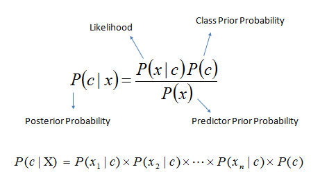
One of the most useful applications of the Bayes rule is the so-called naive Bayes classifier.

The Bayes classifier is a machine learning technique that can be used to classify objects such as text documents into two or more classes. The classifier is trained by analyzing a set of training data, for which the correct classes are given.

The naive Bayes classifier can be used to determine the probabilities of the classes given a number of different observations. The assumption in the model is that the feature variables are conditionally independent given the class (we will not discuss the meaning of conditional independence in this course. For our purposes, it is enough to be able to exploit conditional independence in building the classifier).

Why we call it “naive”

Using spam filters as an example, the idea is to think of the words as being produced by choosing one word after the other so that the choice of the word depends only on whether the message is spam or ham. This is a crude simplification of the process because it means that there is no dependency between adjacent words, and the order of the words has no significance. This is in fact why the method is called naive.

Real world application: spam filters

We will use a spam email filter as a running example for illustrating the idea of the naive Bayes classifier. Thus, the class variable indicates whether a message is spam (or “junk email”) or whether it is a legitimate message (also called “ham”). The words in the message correspond to the feature variables, so that the number of feature variables in the model is determined by the length of the message.

Because the model is based on the idea that the words can be processed independently, we can identify specific words that are indicative of either spam ("FREE", "LAST") or ham ("meeting", "algorithm").

Despite its naivete, the naive Bayes method tends to work very well in practice. This is a good example of the common saying in statistics, “all models are wrong, but some are useful” means (the aphorism is generally attributed to statistician George E.P. Box).

Estimating parameters

To get started, we need to specify the prior odds for spam (against ham). For simplicity assume this to be 1:1 which means that on the average half of the incoming messages are spam (in reality, the amount of spam is probably much higher).

To get our likelihood ratios, we need two different probabilities for any word occurring: one in spam messages and another one in ham messages.

The word distributions for the two classes are best estimated from actual training data that contains some spam messages as well as legitimate messages. The simplest way is to count how many times each word, abacus, acacia, ..., zurg, appears in the data and divide the number by the total word count.

To illustrate the idea, let’s assume that we have at our disposal some spam and some ham. You can easily obtain such data by saving a batch of your emails in two files.

Assume that we have calculated the number of occurrences of the following words (along with all other words) in the two classes of messages:

word	spam	ham
million	156	98
dollars	29	119
adclick	51	0
conferences	0	12
total	95791	306438

We can now estimate that the probability that a word in a spam message is million, for example, is about 156 out of 95791, which is roughly the same as 1 in 614. Likewise, we get the estimate that 98 out of 306438 words, which is about the same as 1 in 3127, in a ham message are million. Both of these probability estimates are small, less than 1 in 500, but more importantly, the former is higher than the latter: 1 in 614 is higher than 1 in 3127. This means that the likelihood ratio, which is the first ratio divided by the second ratio, is more than one. To be more precise, the ratio is (1/614) / (1/3127) = 3127/614 = 5.1 (rounded to one decimal digit).

Zero means trouble

One problem with estimating the probabilities directly from the counts is that zero counts lead to zero estimates. This can be quite harmful for the performance of the classifier – it easily leads to situations where the posterior odds are 0/0, which is nonsense. The simplest solution is to use a small lower bound for all probability estimates. The value 1/100000, for instance, does the job.

Using the above logic, we can determine the likelihood ratio for all possible words without having to use zero, giving us the following likelihood ratios:

word	likelihood ratio
million	5.1
dollars	0.8
adclick	53.2
conferences	0.3

We are now ready to apply the method to classify new messages.

Example: is it spam or ham?

Once we have the prior odds and the likelihood ratios calculated, we are ready to apply the Bayes rule, which we already practiced in the medical diagnosis case as our example. The reasoning goes just like it did before: we update the odds of spam by multiplying it by the likelihood ratio. To remind ourselves of the procedure, let's try a message with a single word to begin with. For the prior odds, as agreed above, you should use odds 1:1.