Bag of Word (BoW) Model

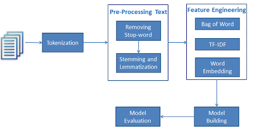
Bag of Word (BoW) Model is used to extract the features from text so that the text can be used in modeling in machine learning algorithms.

Now the question arises that why we need to extract the features from text. It is because the machine learning algorithms cannot work with raw data and they need numeric data so that they can extract meaningful information out of it. The conversion of text data into numeric data is called feature extraction or feature encoding.

This is very simple approach for extracting the features from text. Suppose we have a text document and we want to convert it into numeric data or say want to extract the features out of it then first of all this model extracts a vocabulary from all the words in the document. Then by using a document term matrix, it will build a model. In this way, BoW represents the document as a bag of words only. Any information about the order or structure of words in the document is discarded.

The BoW algorithm builds a model by using the document term matrix. As the name suggests, the document term matrix is the matrix of various word counts that occur in the document. With the help of this matrix, the text document can be represented as a weighted combination of various words. By setting the threshold and choosing the words that are more meaningful, we can build a histogram of all the words in the documents that can be used as a feature vector. Following is an example to understand the concept of document term matrix:

Example

Suppose we have the following two sentences:

• Sentence 1: We are using the Bag of Words model.
• Sentence 2: Bag of Words model is used for extracting the features.

Now, by considering these two sentences, we have the following 13 distinct words:

• we
• are
• using
• the
• bag
• of
• words
• model
• is
• used
• for
• extracting
• features

Now, we need to build a histogram for each sentence by using the word count in each sentence:

Now, we need to build a histogram for each sentence by using the word count in each sentence:

• Sentence 1: [1,1,1,1,1,1,1,1,0,0,0,0,0]
• Sentence 2: [0,0,0,1,1,1,1,1,1,1,1,1,1]

In this way, we have the feature vectors that have been extracted. Each feature vector is 13-dimensional because we have 13 distinct words. Every word is important in the document. The statistics help us understand the importance of every word. The concept of the statistics is called TermFrequency-Inverse Document Frequency (tf-idf).

Term Frequency(tf)

It is the measure of how frequently each word appears in a document. It can be obtained by dividing the count of each word by the total number of words in a given document.

Inverse Document Frequency(idf)

It is the measure of how unique a word is to this document in the given set of documents. For calculating idf and formulating a distinctive feature vector, we need to reduce the weights of commonly occurring words like the and weigh up the rare words.

Building a Bag of Words Model in NLTK

We will define a collection of strings by using CountVectorizer to create vectors from these sentences.
Let us import the necessary package:

from sklearn.feature_extraction.text import CountVectorizer

Now define the set of sentences.

Sentences=['We are using the Bag of Word model', 'Bag of Word model is used for extracting the features.']
vectorizer_count = CountVectorizer()
features_text = vectorizer.fit_transform(Sentences).todense()
print(vectorizer.vocabulary_)

The above program generates the output as shown below. It shows that we have 13 distinct words in the above two sentences:

{'we': 11, 'are': 0, 'using': 10, 'the': 8, 'bag': 1, 'of': 7, 'word': 12, 'model': 6, 'is': 5, 'used': 9, 'for': 4, 'extracting': 2, 'features': 3}

These are the feature vectors (text to numeric form) which can be used for machine learning.

In the next post we'll see how to use this model in solving problems.

Read More

Dividing Data into Chunks: Chunking

The main job of chunking is to identify the parts of speech and short phrases like noun phrases. We have already studied the process of tokenization, the creation of tokens. Chunking basically is the labeling of those tokens. In other words, chunking will show us the structure of the sentence.

There are two types of chunking. The types are as follows:

Chunking up

In this process of chunking, the object, things, etc. move towards being more general and the language gets more abstract. There are more chances of agreement. In this process, we zoom out. For example, if we will chunk up the question that “for what purpose cars are”? We may get the answer “transport”.

Chunking down

In this process of chunking, the object, things, etc. move towards being more specific and the language gets more penetrated. The deeper structure would be examined in chunking down. In this process, we zoom in. For example, if we chunk down the question “Tell specifically about a car”? We will get smaller pieces of information about the car.

Example

In this example, we will do Noun-Phrase chunking, a category of chunking which will find the noun phrases chunks in the sentence, by using the NLTK module in Python:

Follow these steps in python for implementing noun phrase chunking:

• Step 1: In this step, we need to define the grammar for chunking. It would consist of the rules which we need to follow.
• Step 2: In this step, we need to create a chunk parser. It would parse the grammar and give the output.
• Step 3: In this last step, the output is produced in a tree format.

Let us import the necessary NLTK package as follows:

import nltk

Now, we need to define the sentence. Here, DT means the determinant, VBP means the verb, JJ means the adjective, IN means the preposition and NN means the noun.

sentence = [("a", "DT"),("clever", "JJ"),("fox","NN"),("was","VBP"),("jumping","VBP"),("over","IN"),("the","DT"),("wall","NN")]

Now, we need to give the grammar. Here, we will give the grammar in the form of regular expression.

grammar = "NP:{<DT>?<JJ>*<NN>}"

We need to define a parser which will parse the grammar.

parser_chunking=nltk.RegexpParser(grammar)

The parser parses the sentence as follows:

parser_chunking.parse(sentence)

Next, we need to get the output. The output is generated in the simple variable called output_chunk.

Output_chunk=parser_chunking.parse(sentence)

Upon execution of the following code, we can draw our output in the form of a tree.

output.draw()

Read More

Tokenization, Stemming, and Lemmatization

Tokenization

It may be defined as the process of breaking the given text i.e. the character sequence into smaller units called tokens. The tokens may be the words, numbers or punctuation marks. It is also called word segmentation. Following is a simple example of tokenization:

Input: Mango, banana, pineapple and apple all are fruits.

Output:

Mango

Banana
Pineapple
and
Apple
all
are

Fruits

The process of breaking the given text can be done with the help of locating the word boundaries. The ending of a word and the beginning of a new word are called word boundaries. The writing system and the typographical structure of the words influence the boundaries.

In the Python NLTK module, we have different packages related to tokenization which we can use to divide the text into tokens as per our requirements. Some of the packages are as follows:

sent_tokenize package

As the name suggest, this package will divide the input text into sentences. We can import this package with the help of the following Python code:

from nltk.tokenize import sent_tokenize

word_tokenize package

This package divides the input text into words. We can import this package with the help of the following Python code:

from nltk.tokenize import word_tokenize

WordPunctTokenizer package

This package divides the input text into words as well as the punctuation marks. We can import this package with the help of the following Python code:

from nltk.tokenize import WordPuncttokenizer

Stemming

While working with words, we come across a lot of variations due to grammatical reasons. The concept of variations here means that we have to deal with different forms of the same words like democracy, democratic, and democratization. It is very necessary for machines to understand that these different words have the same base form. In this way, it would be useful to extract the base forms of the words while we are analyzing the text.

We can achieve this by stemming. In this way, we can say that stemming is the heuristic process of extracting the base forms of the words by chopping off the ends of words.

In the Python NLTK module, we have different packages related to stemming. These packages can be used to get the base forms of word. These packages use algorithms. Some of the packages are as follows:

PorterStemmer package

This Python package uses the Porter’s algorithm to extract the base form. We can import this package with the help of the following Python code:

from nltk.stem.porter import PorterStemmer

For example, if we will give the word ‘writing’ as the input to this stemmer them we will get the word ‘write’ after stemming.

LancasterStemmer package

This Python package will use the Lancaster’s algorithm to extract the base form. We can import this package with the help of the following Python code:

from nltk.stem.lancaster import LancasterStemmer

For example, if we will give the word ‘writing’ as the input to this stemmer them we will get the word ‘writ’ after stemming.

SnowballStemmer package

This Python package will use the snowball’s algorithm to extract the base form. We can import this package with the help of the following Python code:

from nltk.stem.snowball import SnowballStemmer

For example, if we will give the word ‘writing’ as the input to this stemmer then we will get the word ‘write’ after stemming.

All of these algorithms have different level of strictness. If we compare these three stemmers then the Porter stemmers is the least strict and Lancaster is the strictest. Snowball stemmer is good to use in terms of speed as well as strictness.

Lemmatization

We can also extract the base form of words by lemmatization. It basically does this task with the use of a vocabulary and morphological analysis of words, normally aiming to remove inflectional endings only. This kind of base form of any word is called lemma.

The main difference between stemming and lemmatization is the use of vocabulary and morphological analysis of the words. Another difference is that stemming most commonly collapses derivationally related words whereas lemmatization commonly only collapses the different inflectional forms of a lemma. For example, if we provide the word saw as the input word then stemming might return the word ‘s’ but lemmatization would attempt to return the word either see or saw depending on whether the use of the token was a verb or a noun.

In the Python NLTK module, we have the following package related to lemmatization process which we can use to get the base forms of word:

WordNetLemmatizer package

This Python package will extract the base form of the word depending upon whether it is used as a noun or as a verb. We can import this package with the help of the following Python code:

from nltk.stem import WordNetLemmatizer

Here I am ending this post in which we tried to understand what is tokenization, stemming, and lemmatization. Next post will be on chunking.

Read More

Components of NLP

Natural Language Processing (NLP) refers to AI method of communicating with intelligent systems using a natural language such as English.

Processing of Natural Language is required when you want an intelligent system like robot to perform as per your instructions, when you want to hear decision from a dialogue based clinical expert system, etc.

The field of NLP involves making computers perform useful tasks with the natural languages humans use.

The input and output of an NLP system can be −

• Speech
• Written Text

In this post, we will discuss about the different components of NLP. There are two components of NLP. The components are described below:

Natural Language Understanding (NLU)

It involves the following tasks:

• Mapping the given input in natural language into useful representations.
• Analyzing different aspects of the language.

Natural Language Generation (NLG)

It is the process of producing meaningful phrases and sentences in the form of natural language from some internal representation. It involves:

• Text planning − This includes retrieving the relevant content from the knowledge base.
• Sentence planning − This includes choosing the required words, forming meaningful phrases, setting tone of the sentence.
• Text Realization − This is mapping sentence plan into sentence structure.

Difficulties in NLU

The NLU is very rich in form and structure; however, it is ambiguous. There can be different levels of ambiguity −

Lexical ambiguity

It is at a very primitive level such as the word-level. For example, treating the word “board” as noun or verb?

Syntax level ambiguity

A sentence can be parsed in different ways. For example, “He lifted the beetle with red cap.” − Did he use cap to lift the beetle or he lifted a beetle that had red cap?

Referential ambiguity

Referring to something using pronouns. For example, Rima went to Gauri. She said, “I am tired.” − Exactly who is tired?

NLP Terminology

Let us now see a few important terms in the NLP terminology.

• Phonology − It is study of organizing sound systematically.
• Morphology − It is a study of construction of words from primitive meaningful units.
• Morpheme − It is a primitive unit of meaning in a language.
• Syntax − It refers to arranging words to make a sentence. It also involves determining the structural role of words in the sentence and in phrases.
• Semantics − It is concerned with the meaning of words and how to combine words into meaningful phrases and sentences.
• Pragmatics − It deals with using and understanding sentences in different situations and how the interpretation of the sentence is affected.
• Discourse − It deals with how the immediately preceding sentence can affect the interpretation of the next sentence.
• World Knowledge − It includes the general knowledge about the world.

Steps in NLP

This section shows the different steps in NLP.

Lexical Analysis

It involves identifying and analyzing the structure of words. Lexicon of a language means the collection of words and phrases in a language. Lexical analysis is dividing the whole chunk of txt into paragraphs, sentences, and words.

Syntactic Analysis (Parsing)

It involves analysis of words in the sentence for grammar and arranging words in a manner that shows the relationship among the words. The sentence such as “The school goes to boy” is rejected by English syntactic analyzer.

Semantic Analysis

It draws the exact meaning or the dictionary meaning from the text. The text is checked for meaningfulness. It is done by mapping syntactic structures and objects in the task domain. The semantic analyzer disregards sentence such as “hot ice-cream”.

Discourse Integration

The meaning of any sentence depends upon the meaning of the sentence just before it. In addition, it also brings about the meaning of immediately succeeding sentence.

Pragmatic Analysis

During this, what was said is re-interpreted on what it actually meant. It involves deriving those aspects of language which require real world knowledge.

Read More

Building a KNN classifier

A K-Nearest Neighbors (KNN) classifier is a classification model that uses the nearest neighbors algorithm to classify a given data point. We have implemented the KNN algorithm in the last post, now we are going to build a KNN classifier using that algorithm.

Concept of KNN Classifier

The basic concept of K-nearest neighbor classification is to find a predefined number, i.e., the 'k' - of training samples closest in distance to a new sample, which has to be classified. New samples will get their label from the neighbors itself. The KNN classifiers have a fixed user defined constant for the number of neighbors which have to be determined. For the distance, standard Euclidean distance is the most common choice. The KNN Classifier works directly on the learned samples rather than creating the rules for learning. The KNN algorithm is among the simplest of all machine learning algorithms. It has been quite successful in a large number of classification and regression problems, for example, character recognition or image analysis.

Example

We are building a KNN classifier to recognize digits. For this, we will use the MNIST dataset. We will write this code in the Jupyter Notebook.

Import the necessary packages as shown below.

Here we are using the KNeighborsClassifier module from the sklearn.neighbors package:

from sklearn.datasets import *
import pandas as pd
%matplotlib inline
from sklearn.neighbors import KNeighborsClassifier
import matplotlib.pyplot as plt
import numpy as np

The following code will display the image of digit to verify what image we have to test:

def Image_display(i):
plt.imshow(digit['images'][i],cmap='Greys_r')
plt.show()

Now, we need to load the MNIST dataset. Actually there are total 1797 images but we are using the first 1600 images as training sample and the remaining 197 would be kept for testing purpose.

digit = load_digits()
digit_d = pd.DataFrame(digit['data'][0:1600])

Now, on displaying the images we can see the output as follows:

Image_display(0)

Image_display(0)

Image of 0 is displayed as follows:

Image_display(9)

Image of 9 is displayed as follows:

digit.keys()

Now, we need to create the training and testing data set and supply testing data set to the KNN classifiers.

train_x= digit['data'][:1600]
train_y = digit['target'][:1600]
KNN = KNeighborsClassifier(20)
KNN.fit(train_x,train_y)

The following output will create the K nearest neighbor classifier constructor:

KNeighborsClassifier(algorithm='auto', leaf_size=30, metric='minkowski',
metric_params=None, n_jobs=1, n_neighbors=20, p=2,
weights='uniform')

We need to create the testing sample by providing any arbitrary number greater than 1600, which were the training samples.

test = np.array(digit['data'][1725])
test1 = test.reshape(1,-1)
Image_display(1725)

Image_display(6)

Image of 6 is displayed as follows:

Now we will predict the test data as follows:

KNN.predict(test1)

The above code will generate the following output:

array([6])

Now, consider the following:

digit['target_names']

The above code will generate the following output:

array([0, 1, 2, 3, 4, 5, 6, 7, 8, 9])

In the next post, we will learn about the different components of NLP.

Read More

Finding Nearest Neighbors

If we want to build recommender systems such as a movie recommender system then we need to understand the concept of finding the nearest neighbors. It is because the recommender system utilizes the concept of nearest neighbors.

The concept of finding nearest neighbors may be defined as the process of finding the closest point to the input point from the given dataset. The main use of this KNN (K-nearest neighbors) algorithm is to build classification systems that classify a data point on the proximity of the input data point to various classes.

The Python code given below helps in finding the K-nearest neighbors of a given data set:

Import the necessary packages as shown below. Here, we are using the NearestNeighbors module from the sklearn package:

import numpy as np

import matplotlib.pyplot as plt
from sklearn.neighbors import NearestNeighbors

Let us now define the input data:

A = np.array([[3.1, 2.3], [2.3, 4.2], [3.9, 3.5], [3.7, 6.4], [4.8, 1.9],[8.3, 3.1], [5.2, 7.5], [4.8, 4.7], [3.5, 5.1], [4.4, 2.9],])

Now, we need to define the nearest neighbors:

k = 3

We also need to give the test data from which the nearest neighbors is to be found:

test_data = [3.3, 2.9]

The following code can visualize and plot the input data defined by us:

plt.figure()

plt.title('Input data')

plt.scatter(A[:,0], A[:,1], marker='o', s=100, color='black')

Now, we need to build the K Nearest Neighbor. The object also needs to be trained:

knn_model = NearestNeighbors(n_neighbors=k, algorithm='auto').fit(X)
distances, indices = knn_model.kneighbors([test_data])

Now, we can print the K nearest neighbors as follows:

print("\nK Nearest Neighbors:")
for rank, index in enumerate(indices[0][:k], start=1):
print(str(rank) + " is", A[index])

We can visualize the nearest neighbors along with the test data point:

plt.figure()
plt.title('Nearest neighbors')
plt.scatter(A[:, 0], X[:, 1], marker='o', s=100, color='k')
plt.scatter(A[indices][0][:][:, 0], A[indices][0][:][:, 1],
marker='o', s=250, color='k', facecolors='none')
plt.scatter(test_data[0], test_data[1],
marker='x', s=100, color='k')
plt.show()

Output

K Nearest Neighbors
1 is [ 3.1 2.3]
2 is [ 3.9 3.5]
3 is [ 4.4 2.9]

We have implemented the KNN algorithm, in the next post we are going to build a KNN classifier using this algorithm.

Read More