Pandas - 48 Introduction to TensorFlow framework

TensorFlow is one of the several frameworks in Python that allow you to develop projects for deep learning. This library was developed by the Google Brain Team, a group of Machine Learning Intelligence, a research organization headed by Google.

TensorFlow is already a consolidated deep learning framework, rich in documentation, tutorials, and projects available on the Internet. In addition to the main package, there are many other libraries that have been released over time, including:

• TensorBoard—A kit that allows the visualization of internal graphs to TensorFlow
• TensorFlow Fold—Produces beautiful dynamic calculation charts
• TensorFlow Transform—Created and managed input data pipelines

TensorFlow is based entirely on the structuring and use of graphs and on the flow of data through it, exploiting them in such a way as to make mathematical calculations. The graph created internally to the TensorFlow runtime system is called Data Flow Graph and it is structured in runtime according to the mathematical model that is the basis of the calculation we want to perform. In fact, Tensor Flow allows us to define any mathematical model through a series of instructions implemented in the code.

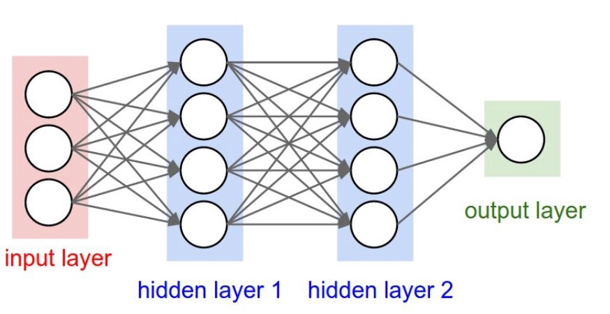
TensorFlow will take care of translating that model into the Data Flow Graph internally. So when we go to model our deep learning neural network, it will be translated into a Data Flow Graph. Given the great similarity between the structure of neural networks and the mathematical representation of graphs, it is easy to understand why this library is excellent for developing deep learning projects.

TensorFlow is not limited to deep learning and can be used to represent artificial neural networks. Many other methods of calculation and analysis can be implemented with this library, since any physical system can be represented with a mathematical model. In fact, this library can also be used to implement other machine learning techniques, and for the study of complex physical systems through the calculation of partial differentials, etc.

The nodes of the Data Flow Graph represent mathematical operations, while the edges of the graph represent tensors (multidimensional data arrays). The name TensorFlow derives from the fact that these tensors represent the flow of data through graphs, which can be used to model artificial neural networks.

Here I am ending today's discussion wherein we covered the basics of TensorFlow framework. In the next post I'll focus on Programming with TensorFlow . So till we meet again keep learning and practicing Python as Python is easy to learn!

Read More

Pandas - 47 Artificial Neural Networks and Deep Learning

Artificial neural networks are a fundamental element for deep learning and their use is the basis of many deep learning techniques. In fact, these systems are able to learn, due to their particular structure that refers to the biological neural circuits.

Artificial neural networks are complex structures created by connecting simple basic components that are repeated within the structure. Depending on the number of these basic components and the type of connections, more and more complex networks will be formed, with different architectures, each of which will present peculiar characteristics regarding the ability to learn and solve different problems of deep learning. The figure below shows how a generic artificial neural network is structured:

The basic units are called nodes (the circles shown in Figure above), which in the biological model simulate the functioning of a neuron within a neural network. These artificial neurons perform very simple operations, similar to the biological counterparts. They are activated when the total sum of the input signals they receive exceeds an activation threshold.

These nodes can transmit signals between them by means of connections, called edges, which simulate the functioning of biological synapses (the arrows shown in Figure above). Through these edges, the signals sent by a neuron pass to the next one, behaving as a filter. That is, an edge converts the output message from a neuron, into an inhibitory or excitant signal, decreasing or increasing its intensity, according to pre-established rules (a different weight is generally applied for each edge).

The neural network has a certain number of nodes used to receive the input signal from the outside (see above Figure ). This first group of nodes is usually represented in a column at the far left end of the neural network schema. This group of nodes represents the first layer of the neural network (input layer). Depending on the input signals received, some (or all) of these neurons will be activated by processing the received signal and transmitting the result as output to another group of neurons, through edges.

This second group is in an intermediate position in the neural network, and is called the hidden layer. This is because the neurons of this group do not communicate with the outside neither in input nor in output and are therefore hidden. As we can see in above Figure, each of these neurons has lots of incoming edges, often with all the neurons of the previous layer. Even these hidden neurons will be activated whether the total incoming signal will exceed a certain threshold. If affirmative, they will process the signal and transmit it to another group of neurons (in the right direction of the scheme shown in above Figure). This group can be another hidden layer or the output layer, that is, the last
layer that will send the results directly to the outside.

Thus we will have a flow of data that will enter the neural network (from left to right), and that will be processed in a more or less complex way depending on the structure, and will produce an output result. The behavior, capabilities, and efficiency of a neural network will depend exclusively on how the nodes are connected and the total number of layers and neurons assigned to each of them. All these factors define the neural network architecture.

Models of neural network

Single Layer Perceptron (SLP)

The Single Layer Perceptron (SLP) is the simplest model of neural network having a two-layer neural
network, without hidden layers, in which a number of input neurons send signals to an output neuron through different connections, each with its own weight. Figure below shows a SLP:

The figure below shows in more detail the inner workings of this type of neural network:

The edges of this structure are represented in this mathematical model by means of a weight vector consisting of the local memory of the neuron.

W = (w1, w2,......, wn)

The output neuron receives an input vector signals xi each coming from a different neuron.

X =(x1, x2,......, xn)

Then it processes the input signals via a weighed sum.



The total signal s is that perceived by the output neuron. If the signal exceeds the activation threshold of the neuron, it will activate, sending 1 as a value, otherwise it will remain inactive, sending -1.







This is the simplest activation function (see function A shown in the below Figure ), we can also use other more complex ones, such as the sigmoid (see function D shown in the below Figure).




Now we have the structure of the SLP neural network ready, let's focus on the learning part now. The learning procedure of a neural network, called the learning phase, works iteratively. That is, a predetermined number of cycles of operation of the neural network are carried out, in each of which the weights of the wi synapses are slightly modified.

Each learning cycle is called an epoch. In order to carry out the learning we will have to use an  appropriate input data, called the training sets. In the training sets, for each input value, the expected output value is obtained. By comparing the output values produced by the neural network with the expected ones we can analyze the differences and modify the weight values, and we can also reduce
them. In practice this is done by minimizing a cost function (loss) that is specific of the problem of deep learning. In fact the weights of the different connections will be modified for each epoch in order to minimize the cost (loss).

In conclusion, supervised learning is applied to neural networks. At the end of the learning phase, we  will pass to the evaluation phase, in which the learned SLP perceptron must analyze another set of inputs (test set) whose results are also known here. By evaluating the differences between the values obtained and those expected, the degree of ability of the neural network to solve the problem of deep
learning will be known. Often the percentage of cases guessed with the wrong ones is used to indicate this value, and it is called accuracy.

Multi Layer Perceptron (MLP)

In this structure, there are one or more hidden layers interposed between the input layer and the output layer. The architecture is represented in Figure shown below:

At the end of the learning phase, we will pass to the evaluation phase, in which the learned SLP perceptron must analyze another set of inputs (test set) whose results are also known here. By evaluating the differences between the values obtained and those expected, the degree of ability of the neural network to solve the problem of deep learning will be known. Often, the percentage of cases guessed with the wrong ones is used to indicate this value, and it is called accuracy.

Although more complex, the models of MLP neural networks are based primarily on the same concepts as the models of the SLP neural networks. Even in MLPs, weights are assigned to each connection. These weights must be minimized based on the evaluation of a training set, much like the SLPs. Here, too, each node must process all incoming signals through an activation function, even if this time the presence of several hidden layers, will make the neural network able to learn more, adapting more effectively to the type of problem deep learning is trying to solve.

From a practical point of view, the greater complexity of this system requires more complex algorithms both for the learning phase and for the evaluation phase. One of these is the back propagation algorithm, used to effectively modify the weights of the various connections to minimize the cost function, in order to quickly and progressively converge the output values with the expected ones. Other algorithms are used specifically for the minimization phase of the cost (or error) function and are generally referred to as gradient descent techniques.

I'd suggest to go into details of these algorithms as we won't discuss about them there.There is also a real correspondence between the two systems at the highest reading level. In fact, we've just seen that neural networks have structures based on layers of neurons. The first layer processes the incoming signal, then passes it to the next layer,which in turn processes it and so on, until it reaches a final result. For each layer of neurons, incoming information is processed in a certain way, generating different levels of representation of the same information.

In fact, the whole operation of elaboration of an artificial neural network is nothing more than the transformation of information to ever more abstract levels. This functioning is identical to what happens in the cerebral cortex. For example, when the eye receives an image, the image signal passes through various processing stages (such as the layers of the neural network), in which, for example, the contours of the figures are first detected (edge detection), then the geometric shape (form perception), and then to the recognition of the nature of the object with its name. Therefore, there has
been a transformation at different levels of conceptuality of an incoming information, passing from an image, to lines, to geometrical figures, to arrive at a word.

Here I am ending today's discussion wherein we covered the basics of artificial neural networks. In the next post I'll focus on the TensorFlow framework . So till we meet again keep learning and practicing Python as Python is easy to learn!

Read More

Pandas - 46 An overview of Deep Learning

Let's have an introductory overview of the world of deep learning and the artificial neural networks on which its techniques are based. Furthermore, among the new Python frameworks for deep  learning, we will use TensorFlow, which is proving to be an excellent tool for research and development of deep learning analysis techniques. With this library we will see how to develop different models of neural networks that are the basis of deep learning.

Artificial intelligence

AI can be defined as

"Automatic processing on a computer capable of performing operations that would seem to be exclusively relevant to human intelligence."

Hence the concept of artificial intelligence is a variable concept that varies with the progress of the machines themselves and with the concept of “exclusive human relevance”.  In the last few years, the concept of artificial intelligence has focused on visual and auditory recognition operations, which until recently were thought of as “exclusive human relevance”. These operations include:

• Image recognition
• Object detection
• Object segmentation
• Language translation
• Natural language understanding
• Speech recognition

Machine learning (ML), with all its techniques and algorithms, is a large branch of artificial intelligence. In fact, you refer to it, while remaining within the ambit of artificial intelligence when you use systems that are able to learn (learning systems) to solve various problems that shortly before had been “considered exclusive to humans”.

Within the machine learning techniques, a further subclass can be defined, called deep learning. We already know that machine learning uses systems that can learn, and this can be done through features inside the system (often parameters of a fixed model) that are modified in response to input data intended for learning (training set).

Deep learning techniques take a step forward. In fact, deep learning systems are structured so as not to have these intrinsic characteristics in the model, but these characteristics are extracted and detected by the system automatically as a result of learning itself. Among these systems that can do this, we refer in particular to artificial neural networks.

The figure below shows the relationship between Artificial Intelligence, Machine
Learning, and Deep Learning:

Deep learning

Deep learning has become popular only in the last few years precisely to solve problems of visual and auditory recognition.

In the context of deep learning, a lot of calculation techniques and algorithms have been developed in recent years, making the most of the potential of the Python language. Thought the theory behind deep learning actually dates back many years, it's only in recent years the neural networks, with the related deep learning techniques that use them, have proved useful to solve many problems of
artificial intelligence.

At the application level, deep learning requires very complex mathematical operations that require millions or even billions of parameters. The CPUs of the 90s, even if powerful, were not able to perform these kinds of operations in efficient times. Even today the calculation with the CPUs, although considerably improved, requires long processing times. This inefficiency is due to the particular architecture of the CPUs, which have been designed to efficiently perform mathematical operations that are not those required by neural networks.

Then Graphics Processing Unit (GPU) were designed to manage more and more efficient vector calculations, such as multiplications between matrices, which is necessary for 3D reality simulations and rendering.

Because of GPU many deep learning techniques have been realized. In fact, to realize the neural networks and their learning, the tensors (multidimensional matrices) are used, carrying out many mathematical operations. It is precisely this kind of work that GPUs are able to do more efficiently. Now the processing speed of deep learning is increased by several orders of magnitude (days instead of months).

Another very important factor affecting the development of deep learning is the huge amount of data that can be accessed. In fact, the data are the fundamental ingredient for the functioning of neural networks, both for the learning phase and for their verification phase. A few years ago only a few organizations were providing data for analysis, today, with the technology such as the IoT (Internet of Things), many sensors and devices acquire data and make them available on networks. Even social networks and search engines (like Facebook, Google, and so on) can collect huge amounts of data,
analyzing in real time millions of users connected to their services (called Big Data).

Thus now a days, a lot of data related to the problems we want to solve with the deep learning techniques, are easily available not only for a fee, but also in free form (open data source).

Python programming language also contributed to the great success and diffusion of deep learning
techniques. In the past, planning neural network systems was very complex. The only language able to carry out this task was C ++, a very complex language, difficult to use and known only to a few specialists. Moreover, in order to work with the GPU (necessary for this type of calculation), it was necessary to know CUDA (Compute Unified Device Architecture), the hardware development architecture of NVIDIA graphics cards with all their technical specifications.

Now because of Python, the programming of neural networks and deep learning techniques has become high level. In fact, programmers no longer have to think about the architecture and the technical specifications of the graphics card (GPU), but can focus exclusively on the part related to deep learning. Moreover the characteristics of the Python language enable programmers to develop simple and intuitive code.

Over the past two years many developer organizations and communities have been developing Python frameworks that are greatly simplifying the calculation and application of deep learning techniques. Among these frameworks available today for free, it is worth mentioning some that
are gaining some success.

• TensorFlow is an open source library for numerical calculation that bases its use on data flow graphs. These are graphs where the nodes represent the mathematical operations and the edges represent tensors (multidimensional data arrays). Its architecture is very flexible and can distribute the calculations both on multiple CPUs and on multiple GPUs.

• Caffe2 is a framework developed to provide an easy and simple way to work on deep learning. It allows you to test model and algorithm calculations using the power of GPUs in the cloud.

• PyTorch is a scientific framework completely based on the use of GPUs. It works in a highly efficient way and was recently developed and is still not well consolidated. It is still proving a powerful tool for scientific research.

• Theano is the most used Python library in the scientific field for the development, definition, and evaluation of mathematical expressions and physical models. Unfortunately, the development team
announced that new versions will no longer be released. However, it remains a reference framework as number of programs were developed with this library, both in literature and on the web.

Here I am ending today's discussion wherein we covered the basics of deep learning. In the next post I'll focus on the artificial neural networks on which its techniques are based. So till we meet again keep learning and practicing Python as Python is easy to learn!

Read More

Pandas - 45 Supervised Learning with scikit-learn (Nonlinear SVC)

In the previous post we have seen the SVC linear algorithm defining a line of separation that was
intended to split the two classes. We have more complex SVC algorithms that can establish curves (2D) or curved surfaces (3D) based on the same principles of maximizing the distances between the points closest to the surface. Let’s see the system using a polynomial kernel. As the name implies, we can define a polynomial curve that separates the area decision in two portions. The degree of the polynomial can be defined by the degree option. Even in this case C is the coefficient of regularization.

In the following program we'll try to apply an SVC algorithm with a polynomial kernel of third degree and with a C coefficient equal to 1:

x = np.array([[1,3],[1,2],[1,1.5],[1.5,2],[2,3],[2.5,1.5],[2,1],[3,1],[3,2],[3.5,1],[3.5,3]])
y = [0]*6 + [1]*5
svc = svm.SVC(kernel='poly',C=1, degree=3).fit(x,y)
X,Y = np.mgrid[0:4:200j,0:4:200j]
Z = svc.decision_function(np.c_[X.ravel(),Y.ravel()])
Z = Z.reshape(X.shape)
plt.contourf(X,Y,Z > 0,alpha=0.4)
plt.contour(X,Y,Z,colors=['k','k','k'], linestyles=['--','-','--'],levels=[-1,0,1])
plt.scatter(svc.support_vectors_[:,0],svc.support_vectors_
[:,1],s=120,facecolors='w')
plt.scatter(x[:,0],x[:,1],c=y,s=50,alpha=0.9)
plt.show()   

The output of the program is shown below which is the decision space using an SVC with a polynomial kernel:

There is another type of nonlinear kernel, the Radial Basis Function (RBF). In this case the
separation curves tend to define the zones radially with respect to the observation points of the training set. See the following program :

x = np.array([[1,3],[1,2],[1,1.5],[1.5,2],[2,3],[2.5,1.5],[2,1],[3,1],[3,2],[3.5,1],[3.5,3]])
y = [0]*6 + [1]*5
svc = svm.SVC(kernel='rbf', C=1, gamma=3).fit(x,y)
X,Y = np.mgrid[0:4:200j,0:4:200j]
Z = svc.decision_function(np.c_[X.ravel(),Y.ravel()])
Z = Z.reshape(X.shape)
plt.contourf(X,Y,Z > 0,alpha=0.4)
plt.contour(X,Y,Z,colors=['k','k','k'], linestyles=['--','-','--'],levels=[-1,0,1])
plt.scatter(svc.support_vectors_[:,0],svc.support_vectors_
[:,1],s=120,facecolors='w')
plt.scatter(x[:,0],x[:,1],c=y,s=50,alpha=0.9)
plt.show()  

The output of the program is shown below in which we can see the two portions of the decision with all points of the training set correctly positioned.:

Now let us use more complex datasets for a classification problem with SVC by using the previously used dataset: the Iris Dataset.

The SVC algorithm used before learned from a training set containing only two classes but now we  will extend the case to three classifications, as the Iris Dataset is split into three classes, corresponding to the three different species of flowers.

In this case the decision boundaries intersect each other, subdividing the decision area (in the case 2D) or the decision volume (3D) in several portions.

Both linear models have linear decision boundaries (intersecting hyperplanes), while models with nonlinear kernels (polynomial or Gaussian RBF) have nonlinear decision boundaries. These boundaries are more flexible with figures that are dependent on the type of kernel and its parameters.
See the following program :

iris = datasets.load_iris()
x = iris.data[:,:2]
y = iris.target
h = .05
svc = svm.SVC(kernel='linear',C=1.0).fit(x,y)
x_min,x_max = x[:,0].min() - .5, x[:,0].max() + .5
y_min,y_max = x[:,1].min() - .5, x[:,1].max() + .5
h = .02
X, Y = np.meshgrid(np.arange(x_min, x_max, h), np.arange(y_min,y_max,h))
Z = svc.predict(np.c_[X.ravel(),Y.ravel()])
Z = Z.reshape(X.shape)
plt.contourf(X,Y,Z,alpha=0.4)
plt.contour(X,Y,Z,colors='k')
plt.scatter(x[:,0],x[:,1],c=y)
plt.show()

The output of the program is shown below where we can see the decision space is divided into three portions separated by decisional boundaries:

Let's apply a nonlinear kernel for generating nonlinear decision boundaries, such as the polynomial kernel as shown in the following program:

iris = datasets.load_iris()
x = iris.data[:,:2]
y = iris.target
h = .05
svc = svm.SVC(kernel='poly',C=1.0,degree=3).fit(x,y)
x_min,x_max = x[:,0].min() - .5, x[:,0].max() + .5
y_min,y_max = x[:,1].min() - .5, x[:,1].max() + .5
h = .02
X, Y = np.meshgrid(np.arange(x_min, x_max, h), np.arange(y_min,y_max,h))
Z = svc.predict(np.c_[X.ravel(),Y.ravel()])
Z = Z.reshape(X.shape)
plt.contourf(X,Y,Z,alpha=0.4)
plt.contour(X,Y,Z,colors='k')
plt.scatter(x[:,0],x[:,1],c=y)
plt.show()   

The output of the program is shown below which shows how the polynomial decision boundaries split the area in a very different way compared to the linear case:

Just notice that in the polynomial case the blue portion is not directly connected with the purple portion. To see the difference in the distribution of areas we can apply the RBF kernel as shown in the following program :

iris = datasets.load_iris()
x = iris.data[:,:2]
y = iris.target
h = .05
svc = svm.SVC(kernel='rbf', gamma=3, C=1.0).fit(x,y)
x_min,x_max = x[:,0].min() - .5, x[:,0].max() + .5
y_min,y_max = x[:,1].min() - .5, x[:,1].max() + .5
h = .02
X, Y = np.meshgrid(np.arange(x_min, x_max, h), np.arange(y_min,y_max,h))
Z = svc.predict(np.c_[X.ravel(),Y.ravel()])
Z = Z.reshape(X.shape)
plt.contourf(X,Y,Z,alpha=0.4)
plt.contour(X,Y,Z,colors='k')
plt.scatter(x[:,0],x[:,1],c=y)
plt.show()    

The output of the program is shown below which shows how the RBF kernel generates radial areas:

We can use the SVC method to solve even regression problems. This method is called Support Vector Regression. The model produced by SVC actually does not depend on the complete training set, but uses only a subset of elements, i.e., those closest to the decisional boundary.

In a similar way, the model produced by SVR also depends only on a subset of the training set. Let's see how the SVR algorithm will use the diabetes dataset that we have already seen in the previous posts. By way of example, we will refer only to the third physiological data. We will perform three different regressions, a linear and two nonlinear (polynomial). The linear case will produce a straight line as the linear predictive model is very similar to the linear regression seen previously, whereas
polynomial regressions will be built of the second and third degrees.

The SVR() function is almost identical to the SVC()function seen previously. The only aspect to consider is that the test set of data must be sorted in ascending order. See the following program :

diabetes = datasets.load_diabetes()
x_train = diabetes.data[:-20]
y_train = diabetes.target[:-20]
x_test = diabetes.data[-20:]
y_test = diabetes.target[-20:]
x0_test = x_test[:,2]
x0_train = x_train[:,2]
x0_test = x0_test[:,np.newaxis]
x0_train = x0_train[:,np.newaxis]
x0_test.sort(axis=0)
x0_test = x0_test*100
x0_train = x0_train*100
svr = svm.SVR(kernel='linear',C=1000)
svr2 = svm.SVR(kernel='poly',C=1000,degree=2)
svr3 = svm.SVR(kernel='poly',C=1000,degree=3)
svr.fit(x0_train,y_train)
svr2.fit(x0_train,y_train)
svr3.fit(x0_train,y_train)
y = svr.predict(x0_test)
y2 = svr2.predict(x0_test)
y3 = svr3.predict(x0_test)
plt.scatter(x0_test,y_test,color='k')
plt.plot(x0_test,y,color='b')
plt.plot(x0_test,y2,c='r')
plt.plot(x0_test,y3,c='g')
plt.show()

The output of the program is shown below:




As shown in the output, the three regression curves will be represented with three colors. The linear
regression will be blue; the polynomial of second degree that is, a parabola, will be red; and the polynomial of third degree will be green.

Here I am ending today’s post. In the next post we shall start with Deep Learning with
TensorFlow. Until we meet again keep practicing and learning Python, as Python is easy to learn!

Read More