Artificial neural networks are a fundamental element for deep learning and their use is the basis of many deep learning techniques. In fact, these systems are able to learn, due to their particular structure that refers to the biological neural circuits.
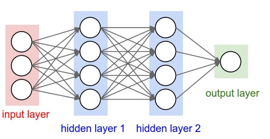
Artificial neural networks are complex structures created by connecting simple basic components that are repeated within the structure. Depending on the number of these basic components and the type of connections, more and more complex networks will be formed, with different architectures, each of which will present peculiar characteristics regarding the ability to learn and solve different problems of deep learning. The figure below shows how a generic artificial neural network is structured:

The basic units are called nodes (the circles shown in Figure above), which in the biological model simulate the functioning of a neuron within a neural network. These artificial neurons perform very simple operations, similar to the biological counterparts. They are activated when the total sum of the input signals they receive exceeds an activation threshold.
These nodes can transmit signals between them by means of connections, called edges, which simulate the functioning of biological synapses (the arrows shown in Figure above). Through these edges, the signals sent by a neuron pass to the next one, behaving as a filter. That is, an edge converts the output message from a neuron, into an inhibitory or excitant signal, decreasing or increasing its intensity, according to pre-established rules (a different weight is generally applied for each edge).
The neural network has a certain number of nodes used to receive the input signal from the outside (see above Figure ). This first group of nodes is usually represented in a column at the far left end of the neural network schema. This group of nodes represents the first layer of the neural network (input layer). Depending on the input signals received, some (or all) of these neurons will be activated by processing the received signal and transmitting the result as output to another group of neurons, through edges.
This second group is in an intermediate position in the neural network, and is called the hidden layer. This is because the neurons of this group do not communicate with the outside neither in input nor in output and are therefore hidden. As we can see in above Figure, each of these neurons has lots of incoming edges, often with all the neurons of the previous layer. Even these hidden neurons will be activated whether the total incoming signal will exceed a certain threshold. If affirmative, they will process the signal and transmit it to another group of neurons (in the right direction of the scheme shown in above Figure). This group can be another hidden layer or the output layer, that is, the last
layer that will send the results directly to the outside.
Thus we will have a flow of data that will enter the neural network (from left to right), and that will be processed in a more or less complex way depending on the structure, and will produce an output result. The behavior, capabilities, and efficiency of a neural network will depend exclusively on how the nodes are connected and the total number of layers and neurons assigned to each of them. All these factors define the neural network architecture.
Models of neural network
Single Layer Perceptron (SLP)
The Single Layer Perceptron (SLP) is the simplest model of neural network having a two-layer neural
network, without hidden layers, in which a number of input neurons send signals to an output neuron through different connections, each with its own weight. Figure below shows a SLP:

The figure below shows in more detail the inner workings of this type of neural network:

The edges of this structure are represented in this mathematical model by means of a weight vector consisting of the local memory of the neuron.
W = (w1, w2,......, wn)
The output neuron receives an input vector signals xi each coming from a different neuron.
X =(x1, x2,......, xn)
Then it processes the input signals via a weighed sum.

The total signal s is that perceived by the output neuron. If the signal exceeds the activation threshold of the neuron, it will activate, sending 1 as a value, otherwise it will remain inactive, sending -1.

This is the simplest activation function (see function A shown in the below Figure ), we can also use other more complex ones, such as the sigmoid (see function D shown in the below Figure).

Now we have the structure of the SLP neural network ready, let's focus on the learning part now. The learning procedure of a neural network, called the learning phase, works iteratively. That is, a predetermined number of cycles of operation of the neural network are carried out, in each of which the weights of the wi synapses are slightly modified.
Each learning cycle is called an epoch. In order to carry out the learning we will have to use an appropriate input data, called the training sets. In the training sets, for each input value, the expected output value is obtained. By comparing the output values produced by the neural network with the expected ones we can analyze the differences and modify the weight values, and we can also reduce
them. In practice this is done by minimizing a cost function (loss) that is specific of the problem of deep learning. In fact the weights of the different connections will be modified for each epoch in order to minimize the cost (loss).
In conclusion, supervised learning is applied to neural networks. At the end of the learning phase, we will pass to the evaluation phase, in which the learned SLP perceptron must analyze another set of inputs (test set) whose results are also known here. By evaluating the differences between the values obtained and those expected, the degree of ability of the neural network to solve the problem of deep
learning will be known. Often the percentage of cases guessed with the wrong ones is used to indicate this value, and it is called accuracy.
Multi Layer Perceptron (MLP)
In this structure, there are one or more hidden layers interposed between the input layer and the output layer. The architecture is represented in Figure shown below:

At the end of the learning phase, we will pass to the evaluation phase, in which the learned SLP perceptron must analyze another set of inputs (test set) whose results are also known here. By evaluating the differences between the values obtained and those expected, the degree of ability of the neural network to solve the problem of deep learning will be known. Often, the percentage of cases guessed with the wrong ones is used to indicate this value, and it is called accuracy.
Although more complex, the models of MLP neural networks are based primarily on the same concepts as the models of the SLP neural networks. Even in MLPs, weights are assigned to each connection. These weights must be minimized based on the evaluation of a training set, much like the SLPs. Here, too, each node must process all incoming signals through an activation function, even if this time the presence of several hidden layers, will make the neural network able to learn more, adapting more effectively to the type of problem deep learning is trying to solve.
From a practical point of view, the greater complexity of this system requires more complex algorithms both for the learning phase and for the evaluation phase. One of these is the back propagation algorithm, used to effectively modify the weights of the various connections to minimize the cost function, in order to quickly and progressively converge the output values with the expected ones. Other algorithms are used specifically for the minimization phase of the cost (or error) function and are generally referred to as gradient descent techniques.
I'd suggest to go into details of these algorithms as we won't discuss about them there.There is also a real correspondence between the two systems at the highest reading level. In fact, we've just seen that neural networks have structures based on layers of neurons. The first layer processes the incoming signal, then passes it to the next layer,which in turn processes it and so on, until it reaches a final result. For each layer of neurons, incoming information is processed in a certain way, generating different levels of representation of the same information.
In fact, the whole operation of elaboration of an artificial neural network is nothing more than the transformation of information to ever more abstract levels. This functioning is identical to what happens in the cerebral cortex. For example, when the eye receives an image, the image signal passes through various processing stages (such as the layers of the neural network), in which, for example, the contours of the figures are first detected (edge detection), then the geometric shape (form perception), and then to the recognition of the nature of the object with its name. Therefore, there has
been a transformation at different levels of conceptuality of an incoming information, passing from an image, to lines, to geometrical figures, to arrive at a word.
Here I am ending today's discussion wherein we covered the basics of artificial neural networks. In the next post I'll focus on the TensorFlow framework . So till we meet again keep learning and practicing Python as Python is easy to learn!
Artificial neural networks are complex structures created by connecting simple basic components that are repeated within the structure. Depending on the number of these basic components and the type of connections, more and more complex networks will be formed, with different architectures, each of which will present peculiar characteristics regarding the ability to learn and solve different problems of deep learning. The figure below shows how a generic artificial neural network is structured:

The basic units are called nodes (the circles shown in Figure above), which in the biological model simulate the functioning of a neuron within a neural network. These artificial neurons perform very simple operations, similar to the biological counterparts. They are activated when the total sum of the input signals they receive exceeds an activation threshold.
These nodes can transmit signals between them by means of connections, called edges, which simulate the functioning of biological synapses (the arrows shown in Figure above). Through these edges, the signals sent by a neuron pass to the next one, behaving as a filter. That is, an edge converts the output message from a neuron, into an inhibitory or excitant signal, decreasing or increasing its intensity, according to pre-established rules (a different weight is generally applied for each edge).
The neural network has a certain number of nodes used to receive the input signal from the outside (see above Figure ). This first group of nodes is usually represented in a column at the far left end of the neural network schema. This group of nodes represents the first layer of the neural network (input layer). Depending on the input signals received, some (or all) of these neurons will be activated by processing the received signal and transmitting the result as output to another group of neurons, through edges.
This second group is in an intermediate position in the neural network, and is called the hidden layer. This is because the neurons of this group do not communicate with the outside neither in input nor in output and are therefore hidden. As we can see in above Figure, each of these neurons has lots of incoming edges, often with all the neurons of the previous layer. Even these hidden neurons will be activated whether the total incoming signal will exceed a certain threshold. If affirmative, they will process the signal and transmit it to another group of neurons (in the right direction of the scheme shown in above Figure). This group can be another hidden layer or the output layer, that is, the last
layer that will send the results directly to the outside.
Thus we will have a flow of data that will enter the neural network (from left to right), and that will be processed in a more or less complex way depending on the structure, and will produce an output result. The behavior, capabilities, and efficiency of a neural network will depend exclusively on how the nodes are connected and the total number of layers and neurons assigned to each of them. All these factors define the neural network architecture.
Models of neural network
Single Layer Perceptron (SLP)
The Single Layer Perceptron (SLP) is the simplest model of neural network having a two-layer neural
network, without hidden layers, in which a number of input neurons send signals to an output neuron through different connections, each with its own weight. Figure below shows a SLP:

The figure below shows in more detail the inner workings of this type of neural network:
The edges of this structure are represented in this mathematical model by means of a weight vector consisting of the local memory of the neuron.
W = (w1, w2,......, wn)
The output neuron receives an input vector signals xi each coming from a different neuron.
X =(x1, x2,......, xn)
Then it processes the input signals via a weighed sum.
The total signal s is that perceived by the output neuron. If the signal exceeds the activation threshold of the neuron, it will activate, sending 1 as a value, otherwise it will remain inactive, sending -1.
This is the simplest activation function (see function A shown in the below Figure ), we can also use other more complex ones, such as the sigmoid (see function D shown in the below Figure).
Now we have the structure of the SLP neural network ready, let's focus on the learning part now. The learning procedure of a neural network, called the learning phase, works iteratively. That is, a predetermined number of cycles of operation of the neural network are carried out, in each of which the weights of the wi synapses are slightly modified.
Each learning cycle is called an epoch. In order to carry out the learning we will have to use an appropriate input data, called the training sets. In the training sets, for each input value, the expected output value is obtained. By comparing the output values produced by the neural network with the expected ones we can analyze the differences and modify the weight values, and we can also reduce
them. In practice this is done by minimizing a cost function (loss) that is specific of the problem of deep learning. In fact the weights of the different connections will be modified for each epoch in order to minimize the cost (loss).
In conclusion, supervised learning is applied to neural networks. At the end of the learning phase, we will pass to the evaluation phase, in which the learned SLP perceptron must analyze another set of inputs (test set) whose results are also known here. By evaluating the differences between the values obtained and those expected, the degree of ability of the neural network to solve the problem of deep
learning will be known. Often the percentage of cases guessed with the wrong ones is used to indicate this value, and it is called accuracy.
Multi Layer Perceptron (MLP)
In this structure, there are one or more hidden layers interposed between the input layer and the output layer. The architecture is represented in Figure shown below:
At the end of the learning phase, we will pass to the evaluation phase, in which the learned SLP perceptron must analyze another set of inputs (test set) whose results are also known here. By evaluating the differences between the values obtained and those expected, the degree of ability of the neural network to solve the problem of deep learning will be known. Often, the percentage of cases guessed with the wrong ones is used to indicate this value, and it is called accuracy.
Although more complex, the models of MLP neural networks are based primarily on the same concepts as the models of the SLP neural networks. Even in MLPs, weights are assigned to each connection. These weights must be minimized based on the evaluation of a training set, much like the SLPs. Here, too, each node must process all incoming signals through an activation function, even if this time the presence of several hidden layers, will make the neural network able to learn more, adapting more effectively to the type of problem deep learning is trying to solve.
From a practical point of view, the greater complexity of this system requires more complex algorithms both for the learning phase and for the evaluation phase. One of these is the back propagation algorithm, used to effectively modify the weights of the various connections to minimize the cost function, in order to quickly and progressively converge the output values with the expected ones. Other algorithms are used specifically for the minimization phase of the cost (or error) function and are generally referred to as gradient descent techniques.
I'd suggest to go into details of these algorithms as we won't discuss about them there.There is also a real correspondence between the two systems at the highest reading level. In fact, we've just seen that neural networks have structures based on layers of neurons. The first layer processes the incoming signal, then passes it to the next layer,which in turn processes it and so on, until it reaches a final result. For each layer of neurons, incoming information is processed in a certain way, generating different levels of representation of the same information.
In fact, the whole operation of elaboration of an artificial neural network is nothing more than the transformation of information to ever more abstract levels. This functioning is identical to what happens in the cerebral cortex. For example, when the eye receives an image, the image signal passes through various processing stages (such as the layers of the neural network), in which, for example, the contours of the figures are first detected (edge detection), then the geometric shape (form perception), and then to the recognition of the nature of the object with its name. Therefore, there has
been a transformation at different levels of conceptuality of an incoming information, passing from an image, to lines, to geometrical figures, to arrive at a word.
Here I am ending today's discussion wherein we covered the basics of artificial neural networks. In the next post I'll focus on the TensorFlow framework . So till we meet again keep learning and practicing Python as Python is easy to learn!
0 comments:
Post a Comment