DataFrames revisited

A DataFrame is an enhanced two-dimensional array. Like Series, DataFrames can have custom row and column indices, and offer additional operations and capabilities that make them more convenient for many data-science oriented tasks. DataFrames also support missing data. Each column in a DataFrame is a  Series. The Series representing each column may contain different element types, as you’ll soon see when we discuss loading datasets into DataFrames.

Let’s create a DataFrame from a dictionary that represents student grades on three exams:

In [1]: import pandas as pd

In [2]: grades_dict = {'Wally': [87, 96, 70],
'Eva': [100, 87, 90],
...: 'Sam': [94, 77, 90], 'Katie': [100, 81,
82],
...: 'Bob': [83, 65, 85]}
...:

In [3]: grades = pd.DataFrame(grades_dict)

In [4]: grades

Out[4]:
Wally Eva Sam Katie Bob
0 87 100 94 100 83
1 96 87 77 81 65
2 70 90 90 82 85

Pandas displays DataFrames in tabular format with the indices left aligned in the index column and the remaining columns’ values right aligned. The dictionary’s keys become the column names and the values associated with each key become the element values in the corresponding column. Shortly, we’ll show how to “flip” the rows and columns. By default, the row indices are auto-generated integers starting from 0. 

We could have specified custom indices with the index keyword argument when we created the DataFrame, as in:

pd.DataFrame(grades_dict, index=['Test1', 'Test2', 'Test3'])

Let’s use the index attribute to change the DataFrame’s indices from sequential integers to labels:

In [5]: grades.index = ['Test1', 'Test2','Test3']

In [6]: grades

Out[6]:
Wally Eva Sam Katie Bob
Test1 87 100 94 100 83
Test2 96 87 77 81 65
Test3 70 90 90 82 85

When specifying the indices, you must provide a one dimensional collection that has the same number of elements as there are rows in the DataFrame; otherwise, a ValueError occurs. Series also provides an index attribute for changing an existing Series’ indices.

One benefit of pandas is that you can quickly and conveniently look at your data in many different ways, including selecting portions of the data. Let’s start by getting Eva’s grades by name, which displays her column as a Series:

In [7]: grades['Eva']

Out[7]:
Test1 100
Test2 87
Test3 90
Name: Eva, dtype: int64

If a DataFrame’s column-name strings are valid Python identifiers, you can use them as attributes. Let’s get Sam’s grades with the Sam attribute:

In [8]: grades.Sam

Out[8]:
Test1 94
Test2 77
Test3 90
Name: Sam, dtype: int64

The next post will focus on Selecting Rows via the loc and iloc Attributes.

Read More

Creating a Series

We can specify custom indices with the index keyword argument:

In [12]: grades = pd.Series([87, 100, 94], index=['Wally', 'Eva', 'Sam'])
In [13]: grades

Out[13]:

Wally 87
Eva 100
Sam 94
dtype: int64

In this case, we used string indices, but you can use other immutable types, including integers not beginning at 0 and nonconsecutive integers. Again, notice how nicely and concisely pandas formats a Series for display.

If you initialize a Series with a dictionary, its keys become the Series’ indices, and its values become the Series’ element values:

In [14]: grades = pd.Series({'Wally': 87, 'Eva':100, 'Sam': 94})
In [15]: grades

Out[15]:
Wally 87
Eva 100
Sam 94
dtype: int64

In a Series with custom indices, you can access individual elements via square brackets containing a custom index value:

In [16]: grades['Eva']

Out[16]: 100

If the custom indices are strings that could represent valid Python identifiers, pandas automatically adds them to the Series as attributes that you can access via a dot (.), as in:

In [17]: grades.Wally

Out[17]: 87

Series also has built-in attributes. For example, the dtype attribute returns the underlying array’s element type:

In [18]: grades.dtype

Out[18]: dtype('int64')

and the values attribute returns the underlying array:

In [19]: grades.values

Out[19]: array([ 87, 100, 94])

If a Series contains strings, you can use its str attribute to call string methods on the elements. First, let’s create a Series of hardware-related strings:

In [20]: hardware = pd.Series(['Hammer', 'Saw','Wrench'])

In [21]: hardware

Out[21]:
0 Hammer
1 Saw
2 Wrench
dtype: object

Note that pandas also right-aligns string element values and that the dtype for strings is object. Let’s call string method contains on each element to determine whether the value of each element contains a
lowercase 'a':

In [22]: hardware.str.contains('a')

Out[22]:
0 True
1 True
2 False
dtype: bool

Pandas returns a Series containing bool values indicating the contains method’s result for each element — the element at index 2 ('Wrench') does not contain an 'a', so its element in the resulting Series is False. Note that pandas handles the iteration internally for you—another example of functional-style programming. The str attribute provides many string-processing methods that are similar to those in
Python’s string type.

The following uses string method upper to produce a new Series containing the uppercase versions of each element in hardware:

In [23]: hardware.str.upper()

Out[23]:
0 HAMMER
1 SAW
2 WRENCH
dtype: object

Read More

Producing Descriptive Statistics for a Series

Series provides many methods for common tasks including producing various descriptive statistics. Here in this post we will see count, mean, min, max and std (standard deviation):

In [6]: grades.count()
Out[6]: 3

In [7]: grades.mean()
Out[7]: 93.66666666666667

In [8]: grades.min()
Out[8]: 87

In [9]: grades.max()
Out[9]: 100

In [10]: grades.std()
Out[10]: 6.506407098647712

Each of these is a functional-style reduction. Calling Series method describe produces all these stats and more:

In [11]: grades.describe()

Out[11]:
count 3.000000
mean 93.666667
std 6.506407
min 87.000000
25% 90.500000
50% 94.000000
75% 97.000000
max 100.000000
dtype: float64

The 25%, 50% and 75% are quartiles:

• 50% represents the median of the sorted values.
• 25% represents the median of the first half of the sorted values. 
• 75% represents the median of the second half of the sorted values.

For the quartiles, if there are two middle elements, then their average is that quartile’s median. We have only three values in our Series, so the 25% quartile is the average of 87 and 94, and the 75% quartile is the average of 94 and 100. Together, the interquartile range is the 75% quartile minus the 25% quartile, which is another measure of dispersion, like standard deviation and variance. Of course, quartiles and interquartile range are more useful in larger datasets.

A large number of methods collectively compute descriptive statistics and other related operations on DataFrame. Most of these are aggregations like sum(), mean(), but some of them, like sumsum(), produce an object of the same size. Generally speaking, these methods take an axis argument, just like ndarray.{sum, std, ...}, but the axis can be specified by name or integer

DataFrame − “index” (axis=0, default), “columns” (axis=1)

Let us create a DataFrame and use this object:

import pandas as pd

import numpy as np

#Create a Dictionary of series

d = {'Name':pd.Series(['Tom','James','Ricky','Vin','Steve','Smith','Jack',

   'Lee','David','Gasper','Betina','Andres']),

   'Age':pd.Series([25,26,25,23,30,29,23,34,40,30,51,46]),

   'Rating':pd.Series([4.23,3.24,3.98,2.56,3.20,4.6,3.8,3.78,2.98,4.80,4.10,3.65])

}

#Create a DataFrame

df = pd.DataFrame(d)

print df

Its output is as follows −

    Age  Name   Rating

0   25   Tom     4.23

1   26   James   3.24

2   25   Ricky   3.98

3   23   Vin     2.56

4   30   Steve   3.20

5   29   Smith   4.60

6   23   Jack    3.80

7   34   Lee     3.78

8   40   David   2.98

9   30   Gasper  4.80

10  51   Betina  4.10

11  46   Andres  3.65

sum()

Returns the sum of the values for the requested axis. By default, axis is index (axis=0).

import pandas as pd

import numpy as np

#Create a Dictionary of series

d = {'Name':pd.Series(['Tom','James','Ricky','Vin','Steve','Smith','Jack',

   'Lee','David','Gasper','Betina','Andres']),

   'Age':pd.Series([25,26,25,23,30,29,23,34,40,30,51,46]),

   'Rating':pd.Series([4.23,3.24,3.98,2.56,3.20,4.6,3.8,3.78,2.98,4.80,4.10,3.65])

}

#Create a DataFrame

df = pd.DataFrame(d)

print df.sum()

Its output is as follows −

Age                                                    382

Name     TomJamesRickyVinSteveSmithJackLeeDavidGasperBe...

Rating                                               44.92

dtype: object

Each individual column is added individually (Strings are appended).

axis=1

This syntax will give the output as shown below.

import pandas as pd

import numpy as np

#Create a Dictionary of series

d = {'Name':pd.Series(['Tom','James','Ricky','Vin','Steve','Smith','Jack',

   'Lee','David','Gasper','Betina','Andres']),

   'Age':pd.Series([25,26,25,23,30,29,23,34,40,30,51,46]),

   'Rating':pd.Series([4.23,3.24,3.98,2.56,3.20,4.6,3.8,3.78,2.98,4.80,4.10,3.65])

}

 

#Create a DataFrame

df = pd.DataFrame(d)

print df.sum(1)

Its output is as follows −

0    29.23

1    29.24

2    28.98

3    25.56

4    33.20

5    33.60

6    26.80

7    37.78

8    42.98

9    34.80

10   55.10

11   49.65

dtype: float64

mean()

Returns the average value

import pandas as pd

import numpy as np

#Create a Dictionary of series

d = {'Name':pd.Series(['Tom','James','Ricky','Vin','Steve','Smith','Jack',

   'Lee','David','Gasper','Betina','Andres']),

   'Age':pd.Series([25,26,25,23,30,29,23,34,40,30,51,46]),

   'Rating':pd.Series([4.23,3.24,3.98,2.56,3.20,4.6,3.8,3.78,2.98,4.80,4.10,3.65])

}

#Create a DataFrame

df = pd.DataFrame(d)

print df.mean()

Its output is as follows −

Age       31.833333

Rating     3.743333

dtype: float64

std()

Returns the Bressel standard deviation of the numerical columns.

import pandas as pd

import numpy as np

#Create a Dictionary of series

d = {'Name':pd.Series(['Tom','James','Ricky','Vin','Steve','Smith','Jack',

   'Lee','David','Gasper','Betina','Andres']),

   'Age':pd.Series([25,26,25,23,30,29,23,34,40,30,51,46]),

   'Rating':pd.Series([4.23,3.24,3.98,2.56,3.20,4.6,3.8,3.78,2.98,4.80,4.10,3.65])

}

#Create a DataFrame

df = pd.DataFrame(d)

print df.std()

Its output is as follows −

Age       9.232682

Rating    0.661628

dtype: float64

Functions & Description

Let us now understand the functions under Descriptive Statistics in Python Pandas. The following table list down the important functions −

Sr.No.	Function	Description
1	count()	Number of non-null observations
2	sum()	Sum of values
3	mean()	Mean of Values
4	median()	Median of Values
5	mode()	Mode of values
6	std()	Standard Deviation of the Values
7	min()	Minimum Value
8	max()	Maximum Value
9	abs()	Absolute Value
10	prod()	Product of Values
11	cumsum()	Cumulative Sum
12	cumprod()	Cumulative Product

Note − Since DataFrame is a Heterogeneous data structure. Generic operations don’t work with all functions.

Functions like sum(), cumsum() work with both numeric and character (or) string data elements without any error. Though n practice, character aggregations are never used generally, these functions do not throw any exception.

Functions like abs(), cumprod() throw exception when the DataFrame contains character or string data because such operations cannot be performed.

Summarizing Data

The describe() function computes a summary of statistics pertaining to the DataFrame columns.

import pandas as pd

import numpy as np

#Create a Dictionary of series

d = {'Name':pd.Series(['Tom','James','Ricky','Vin','Steve','Smith','Jack',

   'Lee','David','Gasper','Betina','Andres']),

   'Age':pd.Series([25,26,25,23,30,29,23,34,40,30,51,46]),

   'Rating':pd.Series([4.23,3.24,3.98,2.56,3.20,4.6,3.8,3.78,2.98,4.80,4.10,3.65])

}

#Create a DataFrame

df = pd.DataFrame(d)

print df.describe()

Its output is as follows −

               Age         Rating

count    12.000000      12.000000

mean     31.833333       3.743333

std       9.232682       0.661628

min      23.000000       2.560000

25%      25.000000       3.230000

50%      29.500000       3.790000

75%      35.500000       4.132500

max      51.000000       4.800000

This function gives the mean, std and IQR values. And, function excludes the character columns and given summary about numeric columns. 'include' is the argument which is used to pass necessary information regarding what columns need to be considered for summarizing. Takes the list of values; by default, 'number'.

object − Summarizes String columns

number − Summarizes Numeric columns

all − Summarizes all columns together (Should not pass it as a list value)

Now, use the following statement in the program and check the output −

import pandas as pd

import numpy as np

#Create a Dictionary of series

d = {'Name':pd.Series(['Tom','James','Ricky','Vin','Steve','Smith','Jack',

   'Lee','David','Gasper','Betina','Andres']),

   'Age':pd.Series([25,26,25,23,30,29,23,34,40,30,51,46]),

   'Rating':pd.Series([4.23,3.24,3.98,2.56,3.20,4.6,3.8,3.78,2.98,4.80,4.10,3.65])

}

#Create a DataFrame

df = pd.DataFrame(d)

print df.describe(include=['object'])

Its output is as follows −

          Name

count       12

unique      12

top      Ricky

freq         1

Now, use the following statement and check the output −

import pandas as pd

import numpy as np

#Create a Dictionary of series

d = {'Name':pd.Series(['Tom','James','Ricky','Vin','Steve','Smith','Jack',

   'Lee','David','Gasper','Betina','Andres']),

   'Age':pd.Series([25,26,25,23,30,29,23,34,40,30,51,46]),

   'Rating':pd.Series([4.23,3.24,3.98,2.56,3.20,4.6,3.8,3.78,2.98,4.80,4.10,3.65])

}

#Create a DataFrame

df = pd.DataFrame(d)

print df. describe(include='all')

Its output is as follows −

          Age          Name       Rating

count   12.000000        12    12.000000

unique        NaN        12          NaN

top           NaN     Ricky          NaN

freq          NaN         1          NaN

mean    31.833333       NaN     3.743333

std      9.232682       NaN     0.661628

min     23.000000       NaN     2.560000

25%     25.000000       NaN     3.230000

50%     29.500000       NaN     3.790000

75%     35.500000       NaN     4.132500

max     51.000000       NaN     4.800000

Read More

pandas Series and DataFrames

 

NumPy’s array is optimized for homogeneous numeric data that’s accessed via integer indices. Data science presents unique demands for which more customized data structures are required. Big data applications must support mixed data types, customized indexing, missing data, data that’s not structured consistently and data that needs to be manipulated into forms appropriate for the databases and data analysis packages you use.

Pandas is the most popular library for dealing with such data. It provides two key collections —Series for one-dimensional collections and DataFrames for two-dimensional collections. You can use pandas’ MultiIndex to manipulate multi-dimensional data in the context of Series and DataFrames.

Wes McKinney created pandas in 2008 while working in industry. The name pandas is derived from the term “panel data,” which is data for measurements over time, such as stock prices or historical temperature readings. McKinney needed a library in which the same data structures could handle both time- and non-time-based data with support for data alignment, missing data, common database-style data manipulations, and more.

NumPy and pandas are intimately related. Series and DataFrames use arrays “under the hood.” Series and DataFrames are valid arguments to many NumPy operations. Similarly, arrays are valid arguments to many Series and DataFrame operations. 

pandas Series

A Series is an enhanced one-dimensional array. Whereas arrays use only zero-based integer indices, Series support custom indexing, including even non-integer indices like strings. Series also offer additional capabilities that make them more convenient for many data-science oriented tasks. For example, Series may have missing data, and many Series operations ignore missing data by default.

By default, a Series has integer indices numbered sequentially from 0. The following creates a Series of
student grades from a list of integers:

In [1]: import pandas as pd
In [2]: grades = pd.Series([87, 100, 94])

The initializer also may be a tuple, a dictionary, an array, another Series or a single value. We’ll show a single value momentarily.

Pandas displays a Series in two-column format with the indices left aligned in the left column and the values right aligned in the right column. After listing the Series elements, pandas shows the data type (dtype) of the underlying array’s elements:

In [3]: grades 

Out[3]:

0 87
1 100
2 94
dtype: int64

Note how easy it is to display a Series in this format, compared to the corresponding code for displaying a list in the same two-column format.

You can create a series of elements that all have the same value:

In [4]: pd.Series(98.6, range(3))

Out[4]:
0 98.6
1 98.6
2 98.6
dtype: float64

The second argument is a one-dimensional iterable object (such as a list, an array or a range) containing the Series’ indices. The number of indices determines the number of elements.

You can access a Series’s elements by via square brackets containing an index:

In [5]: grades[0]

Out[5]: 87

We'll continue with the discussion in next posts.

Read More

Reshaping and Transposing

We’ve used array method reshape to produce two dimensional arrays from one-dimensional ranges. NumPy provides various other ways to reshape arrays.

reshape vs. resize

The array methods reshape and resize both enable you to change an array’s dimensions. Method reshape returns a view (shallow copy) of the original array with the new dimensions. It does not modify the original array:

In [1]: import numpy as np
In [2]: grades = np.array([[87, 96, 70], [100,87, 90]])
In [3]: grades

Out[3]:
array([[ 87, 96, 70],
[100, 87, 90]])

In [4]: grades.reshape(1, 6)

Out[4]: array([[ 87, 96, 70, 100, 87, 90]])

In [5]: grades

Out[5]:
array([[ 87, 96, 70],
[100, 87, 90]])

Method resize modifies the original array’s shape:

In [6]: grades.resize(1, 6)
In [7]: grades

Out[7]: array([[ 87, 96, 70, 100, 87, 90]])

flatten vs. ravel

You can take a multidimensional array and flatten it into a single dimension with the methods flatten and ravel. Method flatten deep copies the original array’s data:

In [8]: grades = np.array([[87, 96, 70], [100,87, 90]])
In [9]: grades

Out[9]:
array([[ 87, 96, 70],
[100, 87, 90]])

In [10]: flattened = grades.flatten()
In [11]: flattened

Out[11]: array([ 87, 96, 70, 100, 87, 90])

In [12]: grades

Out[12]:
array([[ 87, 96, 70],
[100, 87, 90]])

To confirm that grades and flattened do not share the data, let’s modify an element of flattened, then display both arrays:

In [13]: flattened[0] = 100
In [14]: flattened

Out[14]: array([100, 96, 70, 100, 87, 90])

In [15]: grades

Out[15]:
array([[ 87, 96, 70],
[100, 87, 90]])

Method ravel produces a view of the original array, which shares the grades array’s data:

In [16]: raveled = grades.ravel()
In [17]: raveled

Out[17]: array([ 87, 96, 70, 100, 87, 90])

In [18]: grades

Out[18]:
array([[ 87, 96, 70],
[100, 87, 90]])

To confirm that grades and raveled share the same data, let’s modify an element of raveled, then display both arrays:

In [19]: raveled[0] = 100
In [20]: raveled

Out[20]: array([100, 96, 70, 100, 87, 90])

In [21]: grades

Out[21]:
array([[100, 96, 70],
[100, 87, 90]])

Transposing Rows and Columns

You can quickly transpose an array’s rows and columns that is “flip” the array, so the rows become the columns and the columns become the rows. The T attribute returns a transposed view (shallow copy) of the array. The original grades array represents two students’ grades (the rows) on three exams (the columns). Let’s transpose the rows and columns to view the data as the grades on three exams (the
rows) for two students (the columns):

In [22]: grades.T

Out[22]:
array([[100, 100],
[ 96, 87],
[ 70, 90]])

Transposing does not modify the original array:

In [23]: grades

Out[23]:
array([[100, 96, 70],
[100, 87, 90]])

Horizontal and Vertical Stacking

You can combine arrays by adding more columns or more rows—known as horizontal stacking and vertical stacking.

Let’s create another 2-by-3 array of grades:

In [24]: grades2 = np.array([[94, 77, 90], [100,81, 82]])

Let’s assume grades2 represents three additional exam grades for the two students in the grades array. We can combine grades and grades2 with NumPy’s hstack (horizontal stack) function by passing a tuple containing the arrays to combine. The extra parentheses are required because hstack expects one argument:

In [25]: np.hstack((grades, grades2))

Out[25]:
array([[100, 96, 70, 94, 77, 90],
[100, 87, 90, 100, 81, 82]])

Next, let’s assume that grades2 represents two more students’ grades on three exams. In this case, we can combine grades and grades2 with NumPy’s vstack (vertical stack) function:

In [26]: np.vstack((grades, grades2))

Out[26]:
array([[100, 96, 70],
[100, 87, 90],
[ 94, 77, 90],
[100, 81, 82]])

Read More

Deep Copies

 

Though views are separate array objects, they save memory by sharing element data from other arrays. However, when sharing mutable values, sometimes it’s necessary to create a deep copy with independent copies of the original data. This is especially important in multi-core programming, where separate parts of your program could attempt to modify your data at the same time, possibly corrupting it.

The array method copy returns a new array object with a deep copy of the original array object’s data. First, let’s create an array and a deep copy of that array:

In [1]: import numpy as np
In [2]: numbers = np.arange(1, 6)
In [3]: numbers

Out[3]: array([1, 2, 3, 4, 5])

In [4]: numbers2 = numbers.copy()
In [5]: numbers2

Out[5]: array([1, 2, 3, 4, 5])

To prove that numbers2 has a separate copy of the data in numbers, let’s modify an element in numbers, then display both arrays:

In [6]: numbers[1] *= 10
In [7]: numbers

Out[7]: array([ 1, 20, 3, 4, 5])
In [8]: numbers2

Out[8]: array([ 1, 2, 3, 4, 5])

As you can see, the change appears only in numbers.

Read More

Views: Shallow Copies

View objects are objects that “see” the data in other objects, rather than having their own copies of the data. Views are also known as shallow copies. Various array methods and slicing operations produce views of an array’s data.

The array method view returns a new array object with a view of the original array object’s data. First, let’s create an array and a view of that array:

In [1]: import numpy as np
In [2]: numbers = np.arange(1, 6)
In [3]: numbers

Out[3]: array([1, 2, 3, 4, 5])

In [4]: numbers2 = numbers.view()
In [5]: numbers2

Out[5]: array([1, 2, 3, 4, 5]) 

We can use the built-in id function to see that numbers and numbers2 are different objects:

In [6]: id(numbers)
Out[6]: 4462958592

In [7]: id(numbers2)
Out[7]: 4590846240

To prove that numbers2 views the same data as numbers, let’s modify an element in numbers, then display both arrays:

In [8]: numbers[1] *= 10
In [9]: numbers2

Out[9]: array([ 1, 20, 3, 4, 5])
In [10]: numbers

Out[10]: array([ 1, 20, 3, 4, 5])

Similarly, changing a value in the view also changes that value in the original array:

In [11]: numbers2[1] /= 10
In [12]: numbers

Out[12]: array([1, 2, 3, 4, 5])
In [13]: numbers2

Out[13]: array([1, 2, 3, 4, 5])

Slice Views

Slices also create views. Let’s make numbers2 a slice that views only the first three elements of numbers:

In [14]: numbers2 = numbers[0:3]
In [15]: numbers2

Out[15]: array([1, 2, 3])

Again, we can confirm that numbers and numbers2 are different objects with id:

In [16]: id(numbers)

Out[16]: 4462958592

In [17]: id(numbers2)

Out[17]: 4590848000

We can confirm that numbers2 is a view of only the first three numbers elements by attempting to access numbers2[3], which produces an IndexError:

In [18]: numbers2[3]
-------------------------------------------------
------------------------

IndexError Traceback
(most recent call last)
<ipython-input-16-582053f52daa> in <module>()
----> 1 numbers2[3]
IndexError: index 3 is out of bounds for axis 0 with size 3

Now, let’s modify an element both arrays share, then display them. Again, we see that numbers2 is a view of numbers:

In [19]: numbers[1] *= 20
In [20]: numbers

Out[20]: array([1, 2, 3, 4, 5])

In [21]: numbers2
Out[21]: array([ 1, 40, 3])

Read More

Array-Oriented Programming with NumPy- 8 (Indexing and Slicing)

One-dimensional arrays can be indexed and sliced using the same syntax and techniques we use for Lists and Tuples”. Here, we focus on array-specific indexing and slicing capabilities.

Indexing with Two-Dimensional arrays

To select an element in a two-dimensional array, specify a tuple containing the element’s row and column indices in square brackets (as in snippet [4]):

In [1]: import numpy as np
In [2]: grades = np.array([[87, 96, 70], [100, 87, 90],
...: [94, 77, 90], [100,81, 82]])
...:
 

In [3]: grades

Out[3]:
array([[ 87, 96, 70],
[100, 87, 90],
[ 94, 77, 90],
[100, 81, 82]])
 

In [4]: grades[0, 1] # row 0, column 1
Out[4]: 96 

Selecting a Subset of a Two-Dimensional array’s Rows 

To select a single row, specify only one index in square brackets:

In [5]: grades[1]
Out[5]: array([100, 87, 90])

To select multiple sequential rows, use slice notation:

In [6]: grades[0:2]
Out[6]:
array([[ 87, 96, 70],
[100, 87, 90]])

To select multiple non-sequential rows, use a list of row indices:

In [7]: grades[[1, 3]]
Out[7]:
array([[100, 87, 90],
[100, 81, 82]])

Selecting a Subset of a Two-Dimensional array’s Columns

You can select subsets of the columns by providing a tuple specifying the row(s) and column(s) to select. Each can be a specific index, a slice or a list. Let’s select only the elements in the first column:

In [8]: grades[:, 0]
Out[8]: array([ 87, 100, 94, 100])

The 0 after the comma indicates that we’re selecting only column 0. The : before the comma indicates which rows within that column to select. In this case, : is a slice representing all rows. This also could be a specific row number, a slice representing a subset of the rows or a list of specific row indices to select, as in snippets [5]–[7].

You can select consecutive columns using a slice:

In [9]: grades[:, 1:3]
Out[9]:
array([[96, 70],
[87, 90],
[77, 90],
[81, 82]])

or specific columns using a list of column indices:

In [10]: grades[:, [0, 2]]
Out[10]:
array([[ 87, 70],
[100, 90],
[ 94, 90],
[100, 82]])

Read More

Array-Oriented Programming with NumPy- 7 (NumPy Universal Functions)

 

NumPy offers dozens of standalone universal functions (or ufuncs) that perform various element-wise operations. Each performs its task using one or two array or array-like (such as lists) arguments. Some of these functions are called when you use operators like + and * on arrays. Each returns a new array containing the results.

Let’s create an array and calculate the square root of its values, using the sqrt universal function:

In [1]: import numpy as np
In [2]: numbers = np.array([1, 4, 9, 16, 25, 36])

In [3]: np.sqrt(numbers)
Out[3]: array([1., 2., 3., 4., 5., 6.])

Let’s add two arrays with the same shape, using the add universal function:

In [4]: numbers2 = np.arange(1, 7) * 10
In [5]: numbers2
Out[5]: array([10, 20, 30, 40, 50, 60])

In [6]: np.add(numbers, numbers2)
Out[6]: array([11, 24, 39, 56, 75, 96])

The expression np.add(numbers, numbers2) is equivalent to:

numbers + numbers2

Broadcasting with Universal Functions

Let’s use the multiply universal function to multiply every element of numbers2 by the scalar value 5:

In [7]: np.multiply(numbers2, 5)
Out[7]: array([ 50, 100, 150, 200, 250, 300])

The expression np.multiply(numbers2, 5) is equivalent to:

numbers2 * 5

Let’s reshape numbers2 into a 2-by-3 array, then multiply its values by a one-dimensional array of three elements:

In [8]: numbers3 = numbers2.reshape(2, 3)
In [9]: numbers3
Out[9]:
array([[10, 20, 30],
[40, 50, 60]])

In [10]: numbers4 = np.array([2, 4, 6])
In [11]: np.multiply(numbers3, numbers4)
Out[11]:
array([[ 20, 80, 180],
[ 80, 200, 360]])

This works because numbers4 has the same length as each row of numbers3, so NumPy can apply the multiply operation by treating numbers4 as if it were the following array:

array([[2, 4, 6],
[2, 4, 6]])

If a universal function receives two arrays of different shapes that do not support broadcasting, a ValueError occurs. You can view the broadcasting rules at:

https://docs.scipy.org/doc/numpy/user/basics.broadcasting.html

Other Universal Functions

The NumPy documentation lists universal functions in five categories—math, trigonometry, bit manipulation, comparison and floating point. The following table lists some functions from each category. You can view the complete list, their descriptions and more information about universal functions at:

https://docs.scipy.org/doc/numpy/reference/ufuncs.html 

NumPy universal functions

1. Math—add, subtract, multiply, divide, remainder, exp, log,sqrt, power, and more.
2. Trigonometry—sin, cos, tan, hypot, arcsin, arccos, arctan, and more.
3. Bit manipulation—bitwise_and, bitwise_or, bitwise_xor,invert, left_shift and right_shift.
4. Comparison—greater, greater_equal, less, less_equal,equal, not_equal, logical_and, logical_or, logical_xor, logical_not, minimum, maximum, and more.
5. Floating point—floor, ceil, isinf, isnan, fabs, trunc, and more.

Read More

Array-Oriented Programming with NumPy- 6 (NumPy Calculation Methods)

An array has various methods that perform calculations using its contents. By default, these methods ignore the array’s shape and use all the elements in the calculations. For example, calculating the mean of an array totals all of its elements regardless of its shape, then divides by the total number of elements. You can perform these calculations on each dimension as well. For example, in a two-dimensional array, you can calculate each row’s mean and each column’s mean. Consider an array representing four students’ grades on three exams:

In [1]: import numpy as np
In [2]: grades = np.array([[87, 96, 70], [100,87, 90],
...: [94, 77, 90], [100, 81, 82]])
...: 

In [3]: grades
Out[3]:
array([[ 87, 96, 70],
[100, 87, 90],
[ 94, 77, 90],
[100, 81, 82]])

We can use methods to calculate sum, min, max, mean, std (standard deviation) and var (variance)—each is a functional style programming reduction:

In [4]: grades.sum()
Out[4]: 1054

In [5]: grades.min()
Out[5]: 70

In [6]: grades.max()
Out[6]: 100

In [7]: grades.mean()
Out[7]: 87.83333333333333

In [8]: grades.std()
Out[8]: 8.792357792739987

In [9]: grades.var()
Out[9]: 77.30555555555556

Calculations by Row or Column

Many calculation methods can be performed on specific array dimensions, known as the array’s axes. These methods receive an axis keyword argument that specifies which dimension to use in the calculation, giving you a quick way to perform calculations by row or column in a two dimensional
array.

Assume that you want to calculate the average grade on each exam, represented by the columns of grades. Specifying axis=0 performs the calculation on all the row values within each column:

In [10]: grades.mean(axis=0)
Out[10]: array([95.25, 85.25, 83. ])

So 95.25 above is the average of the first column’s grades (87, 100, 94 and 100), 85.25 is the average of the second column’s grades (96, 87, 77 and 81) and 83 is the average of the third column’s grades (70, 90, 90 and 82). Again, NumPy does not display trailing 0s to the right of the decimal point in '83.'. Also note that it does display all element values in the same field width, which is why '83.' is followed by two spaces.

Similarly, specifying axis=1 performs the calculation on all the column values within each individual row. To calculate each student’s average grade for all exams, we can use:

In [11]: grades.mean(axis=1)
Out[11]: array([84.33333333, 92.33333333, 87., 87.66666667])

This produces four averages—one each for the values in each row. So 84.33333333 is the average of row 0’s grades (87, 96 and 70), and the other averages are for the remaining rows. NumPy arrays have many more calculation methods. For the complete list, see https://docs.scipy.org/doc/numpy/reference/
arrays.ndarray.html

Read More

Array-Oriented Programming with NumPy- 5 (array Operators)

NumPy provides many operators which enable you to write simple expressions that perform operations on entire arrays. In this post, I am demonstrating arithmetic between arrays and numeric values and between arrays of the same shape.

Arithmetic Operations with arrays and Individual Numeric Values

First, let’s perform element-wise arithmetic with arrays and numeric values by using arithmetic operators and augmented assignments. Element-wise operations are applied to every element, so snippet [4] multiplies every element by 2 and snippet [5] cubes every element. Each returns a new array
containing the result:

In [1]: import numpy as np
In [2]: numbers = np.arange(1, 6)
In [3]: numbers
Out[3]: array([1, 2, 3, 4, 5]) 

In [4]: numbers * 2
Out[4]: array([ 2, 4, 6, 8, 10])

In [5]: numbers ** 3
Out[5]: array([ 1, 8, 27, 64, 125])

In [6]: numbers # numbers is unchanged by the arithmetic operators
Out[6]: array([1, 2, 3, 4, 5])

Snippet [6] shows that the arithmetic operators did not modify numbers. Operators + and * are commutative, so snippet [4] could also be written as 2 * numbers. 

Augmented assignments modify every element in the left operand.

In [7]: numbers += 10
In [8]: numbers
Out[8]: array([11, 12, 13, 14, 15])

Broadcasting 

Normally, the arithmetic operations require as operands two arrays of the same size and shape. When one operand is a single value, called a scalar, NumPy performs the element wise calculations as if the scalar were an array of the same shape as the other operand, but with the scalar value in all its elements. This is called broadcasting. Snippets [4], [5] and [7] each use this capability. For example, snippet [4] is
equivalent to:

numbers * [2, 2, 2, 2, 2]

Broadcasting also can be applied between arrays of different sizes and shapes, enabling some concise and powerful manipulations. 

Arithmetic Operations Between arrays

You may perform arithmetic operations and augmented assignments between arrays of the same shape. Let’s multiply the one-dimensional arrays numbers and numbers2 (created below) that each contain five elements:

In [9]: numbers2 = np.linspace(1.1, 5.5, 5)
In [10]: numbers2
Out[10]: array([ 1.1, 2.2, 3.3, 4.4, 5.5])

In [11]: numbers * numbers2
Out[11]: array([ 12.1, 26.4, 42.9, 61.6, 82.5])

The result is a new array formed by multiplying the arrays element-wise in each operand—11 * 1.1, 12 * 2.2, 13 *3.3, etc. Arithmetic between arrays of integers and floating-point numbers results in an array of floating-point numbers.

Comparing arrays

You can compare arrays with individual values and with other arrays. Comparisons are performed element-wise. Such comparisons produce arrays of Boolean values in which each element’s True or False value indicates the comparison result:

In [12]: numbers
Out[12]: array([11, 12, 13, 14, 15])

In [13]: numbers >= 13
Out[13]: array([False, False, True, True, True])

In [14]: numbers2
Out[14]: array([ 1.1, 2.2, 3.3, 4.4, 5.5])

In [15]: numbers2 < numbers
Out[15]: array([ True, True, True, True, True])

In [16]: numbers == numbers2
Out[16]: array([False, False, False, False,False])

In [17]: numbers == numbers
Out[17]: array([ True, True, True, True, True])

Snippet [13] uses broadcasting to determine whether each element of numbers is greater than or equal to 13. The remaining snippets compare the corresponding elements of each array operand. 

Read More

Array-Oriented Programming with NumPy-4 (List vs. array Performance)

 

Most array operations execute significantly faster than corresponding list operations. To demonstrate, we’ll use the IPython %timeit magic command, which times the average duration of operations. Note that the times displayed on your system may vary from what we show here.

Timing the Creation of a List Containing Results of 6,000,000 Die Rolls

We’ve demonstrated rolling a six-sided die 6,000,000 times. Here, let’s use the random module’s randrange function with a list comprehension to create a list of six million die rolls and time the operation using %timeit. Note that we used the line-continuation character (\) to split the statement
in snippet [2] over two lines:

In [1]: import random
In [2]: %timeit rolls_list = \
...: [random.randrange(1, 7) for i in
range(0, 6_000_000)]
6.29 s ± 119 ms per loop (mean ± std. dev. of 7 runs, 1 loop each)

By default, %timeit executes a statement in a loop, and it runs the loop seven times. If you do not indicate the number of loops, %timeit chooses an appropriate value. In our testing, operations that on average took more than 500 milliseconds iterated only once, and operations that took fewer than 500
milliseconds iterated 10 times or more.

After executing the statement, %timeit displays the statement’s average execution time, as well as the standard deviation of all the executions. On average, %timeit indicates that it took 6.29 seconds (s) to create the list with a standard deviation of 119 milliseconds (ms). In total, the preceding snippet took about 44 seconds to run the snippet seven times.

Timing the Creation of an array Containing Results of 6,000,000 Die Rolls

Now, let’s use the randint function from the numpy.random module to create an array of 6,000,000
die rolls

In [3]: import numpy as np
In [4]: %timeit rolls_array =
np.random.randint(1, 7, 6_000_000)
72.4 ms ± 635 μs per loop (mean ± std. dev. of 7 runs, 10 loops each)

On average, %timeit indicates that it took only 72.4 milliseconds with a standard deviation of 635 microseconds (μs) to create the array. In total, the preceding snippet took just under half a second to execute on our computer about 1/100th of the time snippet [2] took to execute. The operation is two orders of magnitude faster with array!

60,000,000 and 600,000,000 Die Rolls

Now, let’s create an array of 60,000,000 die rolls:
In [5]: %timeit rolls_array =
np.random.randint(1, 7, 60_000_000)
873 ms ± 29.4 ms per loop (mean ± std. dev. of 7 runs, 1 loop each)

On average, it took only 873 milliseconds to create the array. Finally, let’s do 600,000,000 million die rolls:
In [6]: %timeit rolls_array =
np.random.randint(1, 7, 600_000_000)
10.1 s ± 232 ms per loop (mean ± std. dev. of 7 runs, 1 loop each)

It took about 10 seconds to create 600,000,000 elements with NumPy vs. about 6 seconds to create only 6,000,000 elements with a list comprehension. Based on these timing studies, you can see clearly why
arrays are preferred over lists for compute-intensive operations. In the data science case studies, we’ll enter the performance-intensive worlds of big data and AI. 

Customizing the %timeit Iterations

The number of iterations within each %timeit loop and the number of loops are customizable with the -n and -r options. The following executes snippet [4]’s statement three times per loop and runs the loop twice:
In [7]: %timeit -n3 -r2 rolls_array =
np.random.randint(1, 7, 6_000_000)
85.5 ms ± 5.32 ms per loop (mean ± std. dev. of 2 runs, 3 loops each) 

Other IPython Magics

IPython provides dozens of magics for a variety of tasks for a complete list, see the IPython magics documentation. Here are a few helpful ones:
%load to read code into IPython from a local file or URL.
%save to save snippets to a file.
%run to execute a .py file from IPython.
%precision to change the default floating-point precision for IPython outputs.
%cd to change directories without having to exit IPython first.
%edit to launch an external editor—handy if you need to modify more complex snippets.
%history to view a list of all snippets and commands you’ve executed in the current IPython session.

Read More

Array-Oriented Programming with NumPy-3 (Filling arrays and creating arrays)

NumPy provides functions zeros, ones and full for creating arrays containing 0s, 1s or a specified value,
respectively. By default, zeros and ones create arrays containing float64 values. We’ll show how to customize the element type momentarily. The first argument to these functions must be an integer or a tuple of integers specifying the desired dimensions. For an integer, each function returns a one-dimensional array with the specified number of elements:

In [1]: import numpy as np
In [2]: np.zeros(5)
Out[2]: array([ 0., 0., 0., 0., 0.]) 

For a tuple of integers, these functions return a multidimensional array with the specified dimensions. You can specify the array’s element type with the zeros and ones function’s dtype keyword argument:

In [3]: np.ones((2, 4), dtype=int)
Out[3]: array([[1, 1, 1, 1],
[1, 1, 1, 1]])

The array returned by full contains elements with the second argument’s value and type:

In [4]: np.full((3, 5), 13)
Out[4]:
array([[13, 13, 13, 13, 13],
[13, 13, 13, 13, 13],
[13, 13, 13, 13, 13]])

Creating arrays from Ranges

NumPy provides optimized functions for creating arrays from ranges. We focus on simple evenly spaced integer and floating-point ranges, but NumPy also supports nonlinear ranges. 

a. Creating Integer Ranges with arange

Let’s use NumPy’s arange function to create integer ranges similar to using built-in function range. In each case, arange first determines the resulting array’s number of elements, allocates the memory, then stores the specified range of values in the array:

In [1]: import numpy as np
In [2]: np.arange(5)
Out[2]: array([0, 1, 2, 3, 4])

In [3]: np.arange(5, 10)
Out[3]: array([5, 6, 7, 8, 9])
In [4]: np.arange(10, 1, -2)
Out[4]: array([10, 8, 6, 4, 2])

Though you can create arrays by passing ranges as arguments, always use arange as it’s optimized for arrays.

b. Creating Floating-Point Ranges with linspace

You can produce evenly spaced floating-point ranges with NumPy’s linspace function. The function’s first two arguments specify the starting and ending values in the range, and the ending value is included in the array. The optional keyword argument num specifies the number of evenly spaced values to produce this argument’s default value is 50:

In [5]: np.linspace(0.0, 1.0, num=5)
Out[5]: array([ 0. , 0.25, 0.5 , 0.75, 1. ]) 

c. Reshaping an array

You also can create an array from a range of elements, then use array method reshape to transform the one dimensional array into a multidimensional array. Let’s create an array containing the values from 1 through 20, then reshape it into four rows by five columns:

In [6]: np.arange(1, 21).reshape(4, 5)
Out[6]:
array([[ 1, 2, 3, 4, 5],
[ 6, 7, 8, 9, 10],
[11, 12, 13, 14, 15],
[16, 17, 18, 19, 20]])

Note the chained method calls in the preceding snippet. First, arange produces an array containing the values 1–20. Then we call reshape on that array to get the 4-by-5 array that was displayed. You can reshape any array, provided that the new shape has the same number of elements as the original. So a six-element one-dimensional array can become a 3-by-2 or 2-by-3 array, and vice versa, but attempting to reshape a 15-element array into a 4-by-4 array (16 elements) causes a ValueError.

Displaying Large arrays

When displaying an array, if there are 1000 items or more, NumPy drops the middle rows, columns or both from the output. The following snippets generate 100,000 elements. The first case shows all four rows but only the first and last three of the 25,000 columns. The notation ... represents the missing data. The second case shows the first and last three of the 100 rows, and the first and last three of the 1000 columns:

In [7]: np.arange(1, 100001).reshape(4, 25000)
Out[7]:
array([[ 1, 2, 3, ..., 24998, 24999,
25000],
[ 25001, 25002, 25003, ..., 49998, 49999,
50000],
[ 50001, 50002, 50003, ..., 74998, 74999,
75000],
[ 75001, 75002, 75003, ..., 99998, 99999,
100000]])

In [8]: np.arange(1, 100001).reshape(100, 1000)
Out[8]:
array([[ 1, 2, 3, ..., 998, 999,
1000],
[ 1001, 1002, 1003, ..., 1998, 1999,
2000],
[ 2001, 2002, 2003, ..., 2998, 2999,
3000],
...,
[ 97001, 97002, 97003, ..., 97998, 97999,
98000],
[ 98001, 98002, 98003, ..., 98998, 98999,
99000],
[ 99001, 99002, 99003, ..., 99998, 99999,
100000]])

Read More

Array-Oriented Programming with NumPy-2 (array Attributes)

An array object provides attributes that enable you to discover information about its structure and contents. In this section we’ll use the following arrays:

In [1]: import numpy as np
In [2]: integers = np.array([[1, 2, 3], [4, 5,6]])
In [3]: integers
Out[3]: 

array([[1, 2, 3],
[4, 5, 6]]) 

In [4]: floats = np.array([0.0, 0.1, 0.2, 0.3,0.4])
In [5]: floats
Out[5]: array([ 0. , 0.1, 0.2, 0.3, 0.4])

NumPy does not display trailing 0s to the right of the decimal point in floating-point values.

Determining an array’s Element Type 

The array function determines an array’s element type from its argument’s elements. You can check the element type with an array’s dtype attribute:

In [6]: integers.dtype
Out[6]: dtype('int64') # int32 on some platforms

In [7]: floats.dtype
Out[7]: dtype('float64')

For performance reasons, NumPy is written in the C programming language and uses C’s data types. By default, NumPy stores integers as the NumPy type int64 values which correspond to 64-bit (8-byte) integers in C—and stores floating-point numbers as the NumPy type float64 values which correspond to 64-bit (8-byte) floating-point values in C.

Determining an array’s Dimensions 

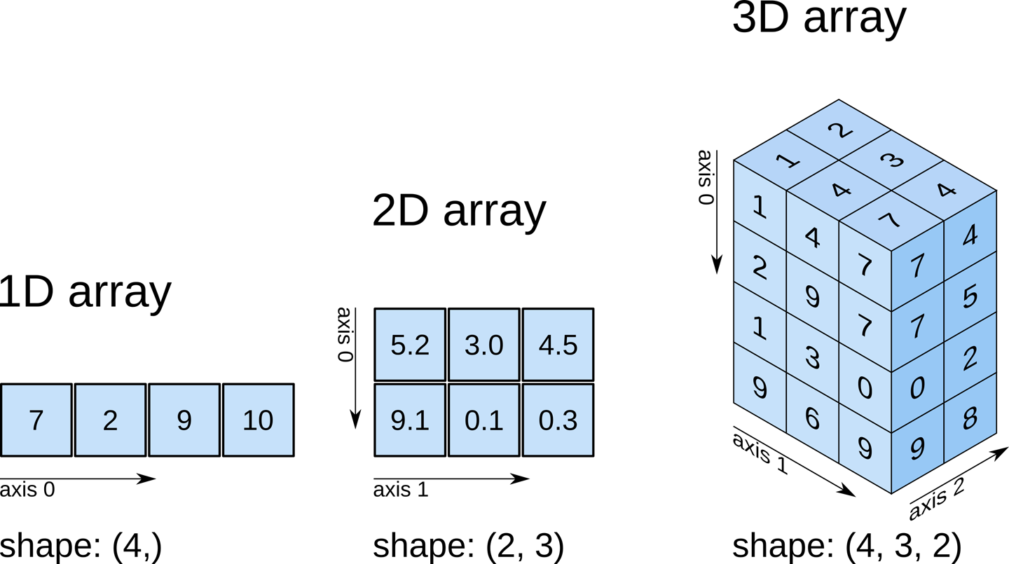
The attribute ndim contains an array’s number of dimensions and the attribute shape contains a tuple
specifying an array’s dimensions:

In [8]: integers.ndim
Out[8]: 2

In [9]: floats.ndim
Out[9]: 1 

In [10]: integers.shape
Out[10]: (2, 3) 

In [11]: floats.shape
Out[11]: (5,) 

Here, integers has 2 rows and 3 columns (6 elements) and floats is one-dimensional, so snippet [11] shows a one element tuple (indicated by the comma) containing floats’ number of elements (5). 

Determining an array’s Number of Elements and Element Size

You can view an array’s total number of elements with the attribute size and the number of bytes required to store each element with itemsize: 

In [12]: integers.size
Out[12]: 6

In [13]: integers.itemsize # 4 if C compiler uses
32-bit ints

Out[13]: 8
In [14]: floats.size 

Out[14]: 5
In [15]: floats.itemsize 

Out[15]: 8

Note that integers’ size is the product of the shape tuple’s values—two rows of three elements each for a total of six elements. In each case, itemsize is 8 because integers contains int64 values and floats contains float64 values, which each occupy 8 bytes.

Iterating Through a Multidimensional array’s Elements

You’ll generally manipulate arrays using concise functional style programming techniques. However, because arrays are iterable, you can use external iteration if you’d like:

In [16]: for row in integers:
...: for column in row:
...: print(column, end=' ')
...: print()
...:
1 2 3
4 5 6 

You can iterate through a multidimensional array as if it were one-dimensional by using its flat attribute:

In [17]: for i in integers.flat:
...: print(i, end=' ')
...:
1 2 3 4 5 6

Read More

Array-Oriented Programming with NumPy-1

The NumPy (Numerical Python) library first appeared in 2006 and is the preferred Python array implementation. It offers a high-performance, richly functional n-dimensional array type called ndarray, which from this point forward we’ll refer to by its synonym, array. NumPy is one of the many opensource libraries that the Anaconda Python distribution installs.

Operations on arrays are up to two orders of magnitude faster than those on lists. In a big-data world in which applications may do massive amounts of processing on vast amounts of array-based data, this performance advantage can be critical. According to libraries.io, over 450 Python libraries depend on NumPy. Many popular data science libraries such as Pandas, SciPy (Scientific Python) and Keras (for deep learning) are built on or depend on NumPy.

Let's explore array’s basic capabilities. Lists can have multiple dimensions. You generally process multidimensional lists with nested loops or list comprehensions with multiple for clauses. A strength of NumPy is “array oriented programming,” which uses functional-style programming with internal iteration to make array manipulations concise and straightforward, eliminating the kinds of bugs that can occur with the external iteration of explicitly programmed loops. 

Creating arrays from Existing Data

The NumPy documentation recommends importing the numpy module as np so that you can access its members with "np.": 

In [1]: import numpy as np

The numpy module provides various functions for creating arrays. Here we use the array function, which receives as an argument an array or other collection of elements and returns a new array containing the argument’s elements. Let’s pass a list:

In [2]: numbers = np.array([2, 3, 5, 7, 11])

The array function copies its argument’s contents into the array. Let’s look at the type of object that function array returns and display its contents:

In [3]: type(numbers)

Out[3]: numpy.ndarray

In [4]: numbers
Out[4]: array([ 2, 3, 5, 7, 11])

Note that the type is numpy.ndarray, but all arrays are output as “array.” When outputting an array, NumPy separates each value from the next with a comma and a space and right-aligns all the values using the same field width. It determines the field width based on the value that occupies the largest number of character positions. In this case, the value 11 occupies the two character positions, so all the values are formatted in two-character fields. That’s why there’s a leading space between the [ and 2. 

Multidimensional Arguments

The array function copies its argument’s dimensions. Let’s create an array from a two-row-by-three-column list:

In [5]: np.array([[1, 2, 3], [4, 5, 6]])
Out[5]:
array([[1, 2, 3],
[4, 5, 6]])

NumPy auto-formats arrays, based on their number of dimensions, aligning the columns within each row. 

We'll continue with arrays in the next post and discuss about array attributes.

Read More

Artificial Intelligence—at the Intersection of CS and Data Science

When a baby first opens its eyes, does it “see” its parent’s faces? Does it understand any notion of what a face is—or even what a simple shape is? Babies must “learn” the world around them. That’s what artificial intelligence (AI) is doing today. It’s looking at massive amounts of data and learning from it. AI is being used to play games, implement a wide range of computer-vision applications, enable self-driving cars, enable robots to learn to perform new tasks, diagnose medical conditions, translate speech to other languages in near real time, create chatbots that can respond to arbitrary questions using massive databases of knowledge, and much more. Who’d have guessed just a few years ago that artificially intelligent self-driving cars would be allowed on our roads—or even become common? Yet, this is now a highly competitive area. The ultimate goal of all this learning is artificial general intelligence—an AI that can perform intelligence tasks as well as humans.

Several artificial-intelligence milestones, in particular, captured people’s attention and imagination, made the general public start thinking that AI is real and made businesses think about commercializing AI: 

1. In a 1997 match between IBM’s DeepBlue computer system and chess Grandmaster Gary Kasparov, DeepBlue became the first computer to beat a reigning world chess champion under tournament conditions. IBM loaded DeepBlue with hundreds of thousands of grandmaster chess games. DeepBlue was capable of using brute force to evaluate up to 200 million moves per second! This is big data at work. IBM received the Carnegie Mellon University Fredkin Prize, which in 1980 offered $100,000 to the creators of the first computer to beat a world chess champion.

2. In 2011, IBM’s Watson beat the two best human Jeopardy! players in a $1 million match. Watson simultaneously used hundreds of language-analysis techniques to locate correct answers in 200 million pages of content (including all of Wikipedia) requiring four terabytes of storage. Watson was trained with machine learning and reinforcement-learning techniques.

3. Go—a board game created in China thousands of years ago —is widely considered to be one of the most complex games ever invented with 10 possible board configurations. To give you a sense of how large a number that is, it’s believed that there are (only) between 10 and 10 atoms in the known universe! In 2015, AlphaGo—created by Google’s DeepMind group—used deep learning with two neural networks to beat the European Go champion Fan Hui. Go is considered to be a far more complex game than chess. 

4. More recently, Google generalized its AlphaGo AI to create AlphaZero—a game-playing AI that teaches itself to play other games. In December 2017, AlphaZero learned the rules of and taught itself to play chess in less than four hours using reinforcement learning. It then beat the world champion chess program, Stockfish 8, in a 100-game match—winning or drawing every game. After training itself in Go for just eight hours, AlphaZero was able to play Go vs. its AlphaGo predecessor, winning 60 of 100 games.

 

 

Read More

Recommendation systems

Recommendation systems are another example of AI technology that has been weaved into our everyday lives. Amazon, YouTube, Netflix, LinkedIn, and Facebook all rely on recommendation technology and we don't even realize we are using it. Recommendation systems rely heavily on data and the more data that is at their disposable, the more powerful they become. It is not coincidence that these companies have some of the biggest market caps in the world and their power comes from them being able to harness the hidden power in their customer's data. Expect this trend to continue in the future.

What is a recommendation? Let's answer the question by first exploring what it is not. It is not a definitive answer. Certain questions like "what is two plus two?" or "how many moons does Saturn have?" have a definite answer and there is no room for subjectivity. Other questions like "what is your favorite movie?" or "do you like radishes?" are completely subjective and the answer is going to depend on the person answering the question. Some machine learning algorithms thrive with this kind of
"fuzziness." Again, these recommendations can have tremendous implications.

Think of the consequences of Amazon constantly recommending a product versus another. The company that makes the recommended product will thrive and the company that makes the product that was not recommended could go out of business if it doesn't find alternative ways to distribute and sell its product.  

One of the ways that a recommender system can improve is by having previous selections from users of the system. If you visit an e-commerce site for the first time and you don't have an order history, the site will have a hard time making a recommendation tailored to you. If you purchase sneakers, the website now has one data point that it can start using as a starting point. Depending on the sophistication of the system, it might recommend a different pair of sneakers, a pair of athletic socks, or maybe even a basketball (if the shoes were high-tops).

An important component of good recommendation systems is a randomization factor that occasionally "goes out on a limb" and makes oddball recommendations that might not be that related to the initial user's choices. Recommender systems don't just learn from history to find similar recommendations, but they also attempt to make new recommendations that might not be related at first blush. For example, a Netflix user might watch "The Godfather" and Netflix might start recommending Al Pacino movies or mobster movies. But it might recommend "Bourne Identity," which is a stretch. If the user does not take the recommendation or does not watch the movie, the algorithm will learn from this and avoid other movies like the "Bourne Identity" (for example any movies that have Jason Bourne as the main character).

As recommender systems get better, the possibilities are exciting. They will be able to power personal digital assistants and become your personal butler that has intimate knowledge of your likes and dislikes and can make great suggestions that you might have not thought about. Some of the areas where recommendations can benefit from these systems are:

• Restaurants
• Movies
• Music
• Potential partners (online dating)
• Books and articles
• Search results
• Financial services (robo-advisors)

Read More