Combinatorial Explosion

At the beginning of a data analysis task, we are tempted to visualize the pairwise interrelationships between all kinds of numeric features that are present in the given dataset. This is often a necessary step for exploratory data analysis and can reveal significant insights about the general pattern of the dataset. However, for large datasets with hundreds of features (columns), this may put extreme pressure on the visualization routine, leading to poor plots and a slow response.

It is easy to explain why this apparently simple (pairwise) scatter plot task can become quickly intractable. The reason is combinatorial explosion. Essentially, you are trying to plot all combinations of two-way relationships and therefore you have nC2 possible combinations to plot where n is the number of numeric features and C denotes the combinatorial sign. Some concrete examples will help.

• 4C2 = 6 so you have 6 plots for pairwise plotting 4 features in a dataset

• 6C2 = 15 so you have 15 plots for pairwise plotting 6 features in a dataset

• 10C2 = 45 so you have 45 plots for pairwise plotting 10 features in a dataset

• 20C2 = 190 so you have 190 plots for pairwise plotting 20 features in a dataset

As you can see in Figure shown below, the number of plots increases rather quickly! On top of that, if you have a large dataset (with millions of samples), then each plot needs to have millions of data points rendered on the screen. It is computationally prohibitive to render millions of points on a web browser for hundreds of plots.

Read More

Iterating Over a pandas DataFrame

Usually we are given a large pandas DataFrame and asked to check some relationships between various fields in the columns, in a row-by-row fashion. It could be a logical operation or a sophisticated mathematical transformation on the raw data.

Essentially, it is a simple case of iterating over the rows of the DataFrame and doing some processing at each iteration. However, it may not be that simple in terms of choosing the most efficient method of executing this apparently simple task. For example, you can choose from the following approaches.

Brute-Force for Loop

The code for this naïve approach will go something like this:

for i in range(len(df)):

if (some condition is satisfied):

<do some calculation with> df.iloc[i]

Essentially, you are iterating over each row (df.iloc[i]) using a generic for loop and processing it one at a time. There’s nothing wrong with the logic and you will get the correct result in the end.

But this is guaranteed to be inefficient. If you try this approach with a DataFrame with a large number of rows, say ~1,000,000 (1 million) and 10 columns, the total iteration may run for tens of seconds or more (even on a fast machine).

Now, you may think that being able to process a million records in tens of seconds is still acceptable. But, as you increase the number of columns or the complexity of the calculation (or of the condition checking done at each iteration), you will see that they quickly add up and this approach should be avoided as much as possible when building scalable DS pipelines. On top of that, if you have to repeat such iteration tasks for hundreds of datasets on a regular basis (in a standard business/production environment), the inefficiencies will stack up over time.

Depending on the situations at hand, you may have choices of two better approaches for this iteration task.

• The pandas library has a dedicated method for iterating over rows named iterrows(), which might be handy to use in this particular situation. Depending on the DataFrame size and the complexity of the row operations, this may reduce the total execution time by ~10X over the for loop approach.

• pandas offers a method for returning a NumPy representation of the DataFrame named df.values(). This can significantly speed things up (even better than iterrows). However, this method removes the axis labels (column names) and therefore you must use the generic NumPy array indexing like 0, 1, to process the data.

We will continue our discussion in the next post

Read More

A Typical Data Science Pipeline

Data science is a vast and dynamic field. In the modern business and technology space, the discipline of data science has assumed the role of a truly transformative force. Every kind of industry and socio-economic field from healthcare to transportation and from online retail to on-demand music uses DS tools and techniques in myriad ways.

Every day exabytes of business and personal data flow through increasingly complex dataflow pipelines architected by sophisticated DataOps architectures to be ingested, processed, and analyzed by database engines or machine learning algorithms, leading to insightful business decisions or technological breakthroughs. However, to illustrate the point of efficient data science practices, let’s take the generic example of a typical data science task flow shown below:

You are probably suspecting that there could be a high chance of writing inefficient code in the data wrangling or ingesting phase. However, you may wonder what could go wrong in the machine learning/statistical modeling phase as you may be using the out-of-the-box methods and routines from highly optimized Python libraries like Scikit-learn, Scipy, or TensorFlow. Furthermore, you may wonder why tasks like quality testing and app deployments should be included in a productive data science pipeline anyway.

Some modules of the DS pipeline in figure shown above, such as data wrangling, visualization, statistical modeling, ML training, and testing, are more directly impacted by inefficient programming styles and practices than others.

In the next posts I'll show some simple examples and take you through some data science stories.

Read More

SQL tables from databases

Spreadsheets share many features with databases, but they are not quite the same. A table extracted from an SQL query from a database can somewhat resemble a spreadsheet. Not surprisingly, spreadsheets can be used to import large amounts of data into a database and a table can be exported from the database in the form of a spreadsheet. But the similarities end there.

Database tables are often the result of an SQL query, which is a series of SQL language statements that allow you to extract, select, and transform the data contained within a database, modifying its format and its original structure to get a data table. Therefore, while the spreadsheets introduce excellent calculation tools applicable to the various areas of the data table, the SQL tables are the result of a complex series of manipulations carried out on original data, based on selections of data of interest from a vast amount of data.

The figure below shows how the SQL Tables started from the characteristics present in the Paper Worksheets, to adapt to relational databases, showing new and powerful properties:

The idea of being able to treat data in memory as if it were an SQL table is incredibly captivating. Likewise, selectively interacting on data selections by applying formulas and calculations as is done with spreadsheets can make the tabular data management powerful.

Well, the pandas library introduced DataFrames as structured data, which makes all this possible. These objects that are the basis of data analysis with Pandas, have an internal tabular structure and are the evolution of the two previous technologies. By combining the calculation features of spreadsheets and the way of working of SQL languages, they provide a new and powerful tool for data analysis. 

The figure below shows how many fundamental properties of Spreadsheets and SQL Tables can be found in the DataFrame, the main data structures of the Pandas library:

Read More

Spreadsheets

A spreadsheet is an application on a computer whose purpose is to organize, analyze, and store data in tabular form. Spreadsheets are nothing more than the digital evolution of paper worksheets. Accountants once collected all the data in large ledgers full of printouts, from which they extracted the accounts. Even the goods in a warehouse were recorded in paper registers made up of rows and columns, in which dates, costs, and various descriptions were reported.

Such a tool has followed the evolution of the times, becoming an office software like spreadsheets, of which the most famous version is precisely Microsoft Excel.

Spreadsheets are programs that operate on data entered in cells within different tables. Each cell can contain both numbers and text strings. With appropriate formulas, you can perform calculations between values contained in areas of selected cells and automatically show the result in another cell. By modifying the values in the operand cells, the value in the cell intended for the result will also be modified in real-time. Spreadsheets, compared to paper worksheets, in addition to organizing the data in tabular form, introduce a certain degree of interaction, in which the user is able to select the data visually, insert calculation formulas, and view the results in real-time.

The figure below shows how Spreadsheets are the digital evolution of Paper Worksheets, adding new useful properties:

Another technology that has enormously marked the evolution of data management is relational databases. We'll discuss about this in the next post.

Read More

Tabular form of data

We know that data must be processed in order to be structured in tabular form. The pandas library also has structured data within it that follow this particular form of ordering the individual data. Now the questions is, why this data structure?

The tabular format has always been the most used method to arrange and organize data. Whether for historical reasons or for a natural predisposition of human rationality to arrange the data in the form of a table, we find the tabular format historically in the collection of the first scientific data written by hand in previous centuries, and in the accountants’ accounts of the first merchants and banks, which in current technologies have internal database tables storing terabytes of data.

Even calendars, recipe ingredients, and other simple things in everyday life follow this structure. The tabular format is simply the information presented in the form of a table with rows and columns, where the data is divided and sorted following the classification logic established by the headings on the rows and columns.

But it is not just a historical question. The reason for the widespread use of this form of organizing data is mainly due to the characteristics that make it ideal for calculating, organizing, and manipulating a large amount of data. They are also easily readable and understandable, even for those with no analysis experience. 

It is no coincidence that most of the software used in offices makes use of tools for entering,  calculating, and saving data in tabular form. A classic example is spreadsheets, of which the most popular of all is Microsoft Excel.

We'll have a quick look at spreadsheets in the next post.

Read More

Remaining steps in the data processing pipeline

Analysis

Analysis is the key step in the data processing pipeline. Here you interpret the raw data, enabling you to draw conclusions that aren’t immediately apparent.

Continuing with our sentiment analysis example, you might want to study the sentiment toward a company over a specified period in relation to that company’s stock price. Or you might compare stock market index figures, such as those on the S&P 500, with the sentiment expressed in a broad sampling of news articles for this same period. The following fragment illustrates what the dataset might look like, with S&P 500 data shown alongside the overall sentiment of that day’s news:

Date News_sentiment S&P_500

---------------------------------------

2021-04-16 0.281074 4185.47

2021-04-19 0.284052 4163.26

2021-04-20 0.262421 4134.94

Since both the sentiment figures and stock figures are expressed in numbers, you might plot two corresponding graphs on the same plot for visual analysis, as illustrated below-

Visual analysis is one of the most commonly used and efficient methods for interpreting data.

Storage

In most cases, you’ll need to store the results generated during the data analysis process to make them available for later use. Your storage options typically include files and databases. The latter is preferable if you anticipate frequent reuse of your data.

Read More

The Data Processing Pipeline

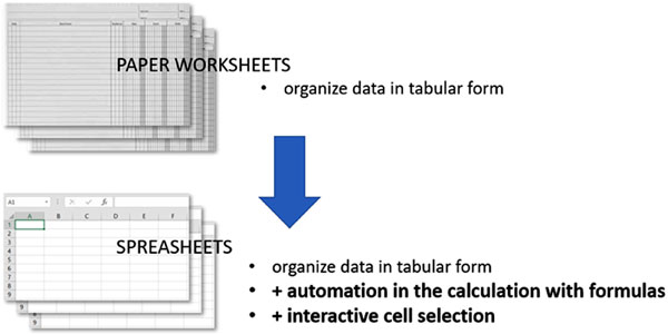
Let's take a conceptual look at the steps involved in data processing, also known as the data processing pipeline. The usual steps applied to the data are:

. Acquisition

. Cleansing

. Transformation

. Analysis

. Storage

You'll notice that these steps aren’t always clear-cut. In some applications you’ll be able to combine multiple steps into one or omit some steps altogether. Now, let's explore these further.

Acquisition

Before you can do anything with data, you need to acquire it. That’s why data acquisition is the first step in any data processing pipeline. We just learned about the most common types of data sources. Some of those sources allow you to load only the required portion of the data in accordance with your request. For example, a request to the Yahoo Finance API requires you to specify the ticker of a company and a period of time over which to retrieve stock prices for that company. Similarly, the News API, which allows you to retrieve news articles, can process a number of parameters to narrow down the list of articles being requested, including the source and date of publication. Despite these qualifying parameters, however, the retrieved list may still need to be filtered further. That is, the data may require cleansing.

Cleansing

Data cleansing is the process of detecting and correcting corrupt or inaccurate data, or removing unnecessary data. In some cases, this step isn’t required, and the data being obtained is immediately ready for analysis. For example, the yfinance library (a Python wrapper for Yahoo Finance API) returns stock data as a readily usable pandas DataFrame object. This usually allows you to skip the cleansing and transformation steps and move straight to data analysis.

However, if your acquisition tool is a web scraper, the data certainly will need cleansing because fragments of HTML markup will probably be included along with the payload data, as shown here:

6.\tThe development shall comply with the requirements of

DCCâ\x80\x99s Drainage Division as follows\r\n\r\n

After cleansing, this text fragment should look like this:

6. The development shall comply with the requirements of

DCC's Drainage Division as follows

Besides the HTML markup, the scraped text may include other unwanted text, as in the following example, where the phrase A View full text is simply hyperlink text. You might need to open this link to access the text within it:

Permission for proposed amendments to planning permission

received on the 30th A View full text

You can also use a data cleansing step to filter out specific entities. After requesting a set of articles from the News API, for example, you may need to select only those articles in the specified period where the titles include a money or percent phrase. This filter can be considered a data cleansing operation because the goal is to remove unnecessary data and prepare for the data transformation and data analysis operations.

Transformation

Data transformation is the process of changing the format or structure of data in preparation for analysis. For example, to extract the information from our GoodComp unstructured text data as we did in “Structured Data,” you might shred it into individual words or tokens so that a named entity recognition (NER) tool can look for the desired information. In information extraction, a named entity typically represents a real-world object, such as a person, an organization, or a product, that can be identified by a proper noun. There are also named entities that represent dates, percentages, financial terms, and more.

Many NLP tools can handle this kind of transformation for you automatically. After such a transformation, the shredded GoodComp data would look like this:

['GoodComp', 'shares', 'soared', 'as', 'much', 'as', '8.2%',

'on',

'2021-01-07', 'after', 'the', 'company', 'announced',

'positive',

'early-stage', 'trial', 'results', 'for', 'its', 'vaccine']

Other forms of data transformation are deeper, with text data being converted into numerical data. For example, if we’ve gathered a collection of news articles, we might transform them by performing sentiment analysis, a text processing technique that generates a number representing the emotions expressed within a text.

Sentiment analysis can be implemented with tools like SentimentAnalyzer, which can be found in the nltk.sentiment package. A typical analysis output might look like this:

Sentiment URL

--------- --------------------------------------------------

--------------

0.9313 https://mashable.com/uk/shopping/amazon-face-maskstore-

july-28/

0.9387 https://skillet.lifehacker.com/save-thosecrustacean-

shells-to

-make-a-sauce-base-1844520024

Each entry in our dataset now includes a number, such as 0.9313, representing the sentiment expressed within the corresponding article. With the sentiment of each article expressed numerically, we can calculate the average sentiment of the entire dataset, allowing us to determine the overall sentiment toward an object of interest, such as a certain company or product.

We'll continue our discussion over remaining steps in the next post

Read More

Files

Files may contain structured, semistructured, and unstructured data. Python’s built-in open() function allows you to open a file so you can use its data within your script. However, depending on the format of the data (for example, CSV, JSON, or XML), you may need to import a corresponding library to be able to perform read, write, and/or append operations on it.

Plaintext files don’t require a library to be further processed and are simply considered as sequences of lines in Python. As an example, look at the following message that a Cisco router might send to a logfile:

dat= 'Jul 19 10:30:37'

host='sm1-prt-highw157'

syslogtag='%SYS-1-CPURISINGTHRESHOLD:'

msg=' Threshold: Total CPU Utilization(Total/Intr): 17%/1%,

Top 3 processes(Pid/Util): 85/9%, 146/4%, 80/1%'

You’ll be able to read this line by line, looking for the required information. Thus, if your task is to find messages that include information about CPU utilization and extract particular figures from it, your script should recognize the last line in the snippet as a message to be selected.

Read More

Databases

Another common source of data is a relational database, a structure that provides a mechanism to efficiently store, access, and manipulate your structured data. You fetch from or send a portion of data to tables in the database using a Structured Query Language (SQL) request. For instance, the following request issued to an employees table in the database retrieves the list of only those programmers who work in the IT department, making it unnecessary to fetch the entire table:

SELECT first_name, last_name FROM employees WHERE department= 'IT' and title = 'programmer'

Python has a built-in database engine, SQLite. Alternatively, you can employ any other available database. Before you can access a database, you’ll need to install the database client software in your environment.

In addition to the conventional rigidly structured databases, there’s been an ever-increasing need in recent years for the ability to store heterogeneous and unstructured data in database-like containers. This has led to the rise of so-called NoSQL (non-SQL or not only SQL) databases. NoSQL databases use flexible data models, allowing you to store large volumes of unstructured data using the key-value method, where each piece of data can be accessed using an associated key. Here’s what our earlier sample financial statement might look like if stored in a NoSQL database:

key value

--- -----

...

26  GoodComp shares soared as much as 8.2% on 2021-01-07 after the company announced ...

The entire statement is paired with an identifying key, 26. It might seem odd to store the entire statement in a database. Recall, however, that several possible records can be extracted from a single statement. Storing the whole statement gives us the flexibility to extract different pieces of information at a later time.

In the next post we shall look into another source which is Files

Read More