About predicting the future - how AI will transform our lives

While some forecasts will probably get at least something right, others will likely be useful only as demonstrations of how hard it is to predict, and many don’t make much sense. What we would like to achieve is for you to be able to look at these and other forecasts, and be able to critically evaluate them.

On hedgehogs and foxes

The political scientist Philip E. Tetlock, author of Superforecasting: The Art and Science of Prediction, classifies people into two categories: those who have one big idea (“hedgehogs”), and those who have many small ideas (“foxes”). Tetlock has carried out an experiment between 1984 and 2003 to study factors that could help us identify which predictions are likely to be accurate and which are not. One of the significant findings was that foxes tend to be clearly better at prediction than hedgehogs, especially when it comes to long-term forecasting.

Probably the messages that can be expressed in 280 characters are more often big and simple hedgehog ideas. Our advice is to pay attention to carefully justified and balanced information sources, and to be suspicious about people who keep explaining everything using a single argument.

Predicting the future is hard but at least we can consider the past and present AI, and by understanding them, hopefully be better prepared for the future, whatever it turns out to be like.

AI winters

The history of AI, just like many other fields of science, has witnessed the coming and going of various different trends. In philosophy of science, the term used for a trend is paradigm. Typically, a particular paradigm is adopted by most of the research community and optimistic predictions about progress in the near-future are provided. For example, in the 1960s neural networks were widely believed to solve all AI problems by imitating the learning mechanisms in the nature, the human brain in particular. The next big thing was expert systems based on logic and human-coded rules, which was the dominant paradigm in the 1980s.

The cycle of hype

In the beginning of each wave, a number of early success stories tend to make everyone happy and optimistic. The success stories, even if they may be in restricted domains and in some ways incomplete, become the focus on public attention. Many researchers rush into AI – or at least calling their research AI – in order to access the increased research funding. Companies also initiate and expand their efforts in AI in the fear of missing out (FOMO).

So far, each time an all-encompassing, general solution to AI has been said to be within reach, progress has ended up running into insurmountable problems, which at the time were thought to be minor hiccups. In the case of neural networks in the 1960s, the hiccups were related to handling nonlinearities and to solving the machine learning problems associated with the increasing number of parameters required by neural network architectures. In the case of expert systems in the 1980s, the hiccups were associated with handling uncertainty and common sense. As the true nature of the remaining problems dawned after years of struggling and unsatisfied promises, pessimism about the paradigm accumulated and an AI winter followed: interest in the field faltered and research efforts were directed elsewhere.

Modern AI

Currently, roughly since the turn of the millennium, AI has been on the rise again. Modern AI methods tend to focus on breaking a problem into a number of smaller, isolated and well-defined problems and solving them one at a time. Modern AI is bypassing grand questions about meaning of intelligence, the mind, and consciousness, and focusing on building practically useful solutions in real-world problems. Good news for us all who can benefit from such solutions!

Another characteristic of modern AI methods, closely related to working in the complex and “messy” real world, is the ability to handle uncertainty, which we demonstrated by studying the uses of probability in AI. Finally, the current upwards trend of AI has been greatly boosted by the come-back of neural networks and deep learning techniques capable of processing images and other real-world data better than anything we have seen before.

Read More

Generative adversarial networks (GANs)

Having learned a neural network from data, it can be used for prediction. Since the top layers of the network have been trained in a supervised manner to perform a particular classification or prediction task, the top layers are really useful only for that task. A network trained to detect stop signs is useless for detecting handwritten digits or cats.

A fascinating result is obtained by taking the pre-trained bottom layers and studying what the features they have learned look like. This can be achieved by generating images that activate a certain set of neurons in the bottom layers. Looking at the generated images, we can see what the neural network “thinks” a particular feature looks like, or what an image with a select set of features in it would look like. Some even like to talk about the networks “dreaming” or “hallucinating” images.

To actually generate real looking cats, human faces, or other objects (you’ll get whatever you used as the training data), Ian Goodfellow who currently works at Google Brain, proposed a clever combination of two neural networks. The idea is to let the two networks compete against each other. One of the networks is trained to generate images like the ones in the training data. The other network’s task is to separate images generated by the first network from real images from the training data – it is called the adversarial network, and the whole system is called generative adversarial network or a GAN.

The system trains the two models side by side. In the beginning of the training, the adversarial model has an easy task to tell apart the real images from the training data and the clumsy attempts by the generative model. However, as the generative network slowly gets better and better, the adversarial model has to improve as well, and the cycle continues until eventually the generated images are almost indistinguishable from real ones. The GAN tries to not only reproduce the images in the training data: that would be a way too simple strategy to beat the adversarial network. Rather, the system is trained so that it has to be able to generate new, real-looking images too.

Read More

Convolutional neural networks (CNNs)

Why we need CNNs

CNNs use a clever trick to reduce the amount of training data required to detect objects in different conditions. The trick basically amounts to using the same input weights for many neurons – so that all of these neurons are activated by the same pattern – but with different input pixels. We can for example have a set of neurons that are activated by a cat’s pointy ear. When the input is a photo of a cat, two neurons are activated, one for the left ear and another for the right. We can also let the neuron’s input pixels be taken from a smaller or a larger area, so that different neurons are activated by the ear appearing in different scales (sizes), so that we can detect a small cat's ears even if the training data only included images of big cats.

One area where deep learning has achieved spectacular success is image processing. The simple classifier that we studied in detail in the previous section is severely limited – as you noticed it wasn't even possible to classify all the smiley faces correctly. Adding more layers in the network and using backpropagation to learn the weights does in principle solve the problem, but another one emerges: the number of weights becomes extremely large and consequently, the amount of training data required to achieve satisfactory accuracy can become too large to be realistic.

Fortunately, a very elegant solution to the problem of too many weights exists: a special kind of neural network, or rather, a special kind of layer that can be included in a deep neural network. This special kind of layer is a so-called convolutional layer. Networks including convolutional layers are called convolutional neural networks (CNNs). Their key property is that they can detect image features such as bright or dark (or specific color) spots, edges in various orientations, patterns, and so on. These form the basis for detecting more abstract features such as a cat’s ears, a dog’s snout, a person’s eye, or the octagonal shape of a stop sign. It would normally be hard to train a neural network to detect such features based on the pixels of the input image, because the features can appear in different positions, different orientations, and in different sizes in the image: moving the object or the camera angle will change the pixel values dramatically even if the object itself looks just the same to us. In order to learn to detect a stop sign in all these different conditions would require vast of amounts of training data because the network would only detect the sign in conditions where it has appeared in the training data. So, for example, a stop sign in the top right corner of the image would be detected only if the training data included an image with the stop sign in the top right corner. CNNs can recognize the object anywhere in the image no matter where it has been observed in the training images.

The convolutional neurons are typically placed in the bottom layers of the network, which processes the raw input pixels. Basic neurons (like the perceptron neuron discussed above) are placed in the higher layers, which process the output of the bottom layers. The bottom layers can usually be trained using unsupervised learning, without a particular prediction task in mind. Their weights will be tuned to detect features that appear frequently in the input data. Thus, with photos of animals, typical features will be ears and snouts, whereas in images of buildings, the features are architectural components such as walls, roofs, windows, and so on. If a mix of various objects and scenes is used as the input data, then the features learned by the bottom layers will be more or less generic. This means that pre-trained convolutional layers can be reused in many different image processing tasks. This is extremely important since it is easy to get virtually unlimited amounts of unlabeled training data – images without labels – which can be used to train the bottom layers. The top layers are always trained by supervised machine learning techniques such as backpropagation.

Read More

A simple neural network classifier

To give a relatively simple example of using a neural network classifier, we'll consider a task that is very similar to the MNIST digit recognition task, namely classifying images in two classes. We will first create a classifier to classify whether an image shows a cross (x) or a circle (o). Our images are represented here as pixels that are either colored or white, and the pixels are arranged in 5 × 5 grid. In this format our images of a cross and a circle (more like a diamond, to be honest) look like this:

In order to build a neural network classifier, we need to formalize the problem in a way where we can solve it using the methods we have learned. Our first step is to represent the information in the pixels by numerical values that can be used as the input to a classifier. Let's use 1 if the square is colored, and 0 if it is white. Note that although the symbols in the above graphic are of different color (green and blue), our classifier will ignore the color information and use only the colored/white information. The 25 pixels in the image make the inputs of our classifier.

To make sure that we know which pixel is which in the numerical representation, we can decide to list the pixels in the same order as you'd read text, so row by row from the top, and reading each row from left to right. The first row of the cross, for example, is represented as 1,0,0,0,1; the second row as 0,1,0,1,0, and so on. The full input for the cross input is then: 1,0,0,0,1,0,1,0,1,0,0,0,1,0,0,0,1,0,1,0,1,0,0,0,1.

We'll use the basic neuron model where the first step is to compute a linear combination of the inputs. Thus need a weight for each of the input pixels, which means 25 weights in total.

Finally, we use the step activation function. If the linear combination is negative, the neuron activation is zero, which we decide to use to signify a cross. If the linear combination is positive, the neuron activation is one, which we decide to signify a circle.

Let's try what happens when all the weights take the same numerical value, 1. With this setup, our linear combination for the cross image will be 9 (9 colored pixels, so 9 × 1, and 16 white pixels, 16 × 0), and for the circle image it will be 8 (8 colored pixels, 8 × 1, and 17 white pixels, 17 × 0). In other words, the linear combination is positive for both images and they are thus classified as circles. Not a very good result given that there are only two images to classify.

To improve the result, we need to adjust the weights in such a way that the linear combination will be negative for a cross and positive for a circle. If we think about what differentiates images of crosses and circles, we can see that circles have no colored pixels in the center of the image, whereas crosses do. Likewise, the pixels at the corners of the image are colored in the cross, but white in the circle.

We can now adjust the weights. There are an infinite number of weights that do the job. For example, assign weight -1 to the center pixel (the 13th pixel), and weight 1 to the pixels in the middle of each of the four sides of the image, letting all the other weights be 0. Now, for the cross input, the center pixel produce the value –1, while for all the other pixels either the pixel value or the weight is 0, so that –1 is also the total value. This leads to activation 0, and the cross is correctly classified.

How about the circle then? Each of the pixels in the middle of the sides produces the value 1, which makes 4 × 1 = 4 in total. For all the other pixels either the pixel value or the weight is zero, so 4 is the total. Since 4 is a positive value, the activation is 1, and the circle is correctly recognized as well.

Read More

Putting neurons together: networks

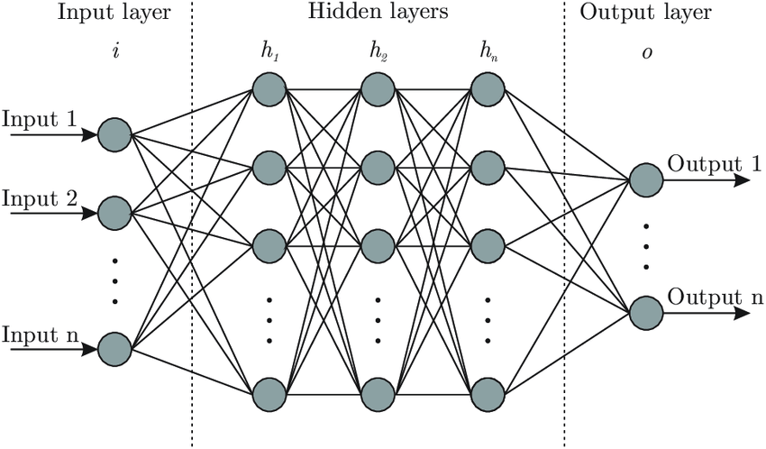
A single neuron would be way too simple to make decisions and prediction reliably in most real-life applications. To unleash the full potential of neural networks, we can use the output of one neuron as the input of other neurons, whose outputs can be the input to yet other neurons, and so on. The output of the whole network is obtained as the output of a certain subset of the neurons, which are called the output layer.

Layers

Often the network architecture is composed of layers. The input layer consists of neurons that get their inputs directly from the data. So for example, in an image recognition task, the input layer would use the pixel values of the input image as the inputs of the input layer. The network typically also has hidden layers that use the other neurons´ outputs as their input, and whose output is used as the input to other layers of neurons. Finally, the output layer produces the output of the whole network. All the neurons on a given layer get inputs from neurons on the previous layer and feed their output to the next.

A classical example of a multilayer network is the so-called multilayer perceptron. As we discussed above, Rosenblatt’s Perceptron algorithm can be used to learn the weights of a perceptron. For multilayer perceptron, the corresponding learning problem is way harder and it took a long time before a working solution was discovered. But eventually, one was invented: the backpropagation algorithm lead to a revival of neural networks in the late 1980s. It is still at the heart of many of the most advanced deep learning solutions.

The path(s) leading to the backpropagation algorithm are rather long and winding. An interesting part of the history is related to the computer science department of the University of Helsinki. About three years after the founding of the department in 1967, a Master’s thesis was written by a student called Seppo Linnainmaa. The topic of the thesis was “Cumulative rounding error of algorithms as a Taylor approximation of individual rounding errors” (the thesis was written in Finnish, so this is a translation of the actual title “Algoritmin kumulatiivinen pyöristysvirhe yksittäisten pyöristysvirheiden Taylor-kehitelmänä”).

The automatic differentiation method developed in the thesis was later applied by other researchers to quantify the sensitivity of the output of a multilayer neural network with respect to the individual weights, which is the key idea in backpropagation.

Read More

Perceptron: the mother of all ANNs

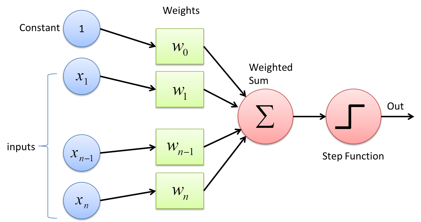
The perceptron is simply a fancy name for the simple neuron model with the step activation function we discussed before. It was among the very first formal models of neural computation and because of its fundamental role in the history of neural networks, it wouldn’t be unfair to call it the “mother of all artificial neural networks”.

It can be used as a simple classifier in binary classification tasks. A method for learning the weights of the perceptron from data, called the Perceptron algorithm, was introduced by the psychologist Frank Rosenblatt in 1957. We will not study the Perceptron algorithm in detail. Suffice to say that it is just about as simple as the nearest neighbor classifier. The basic principle is to feed the network training data one example at a time. Each misclassification leads to an update in the weight.

The history of the debate that eventually lead to almost complete abandoning of the neural network approach in the 1960s for more than two decades is extremely fascinating. The article A Sociological Study of the Official History of the Perceptrons Controversy by Mikel Olazaran (published in Social Studies of Science, 1996) reviews the events from a sociology of science point of view. Reading it today is quite thought provoking. Reading stories about celebrated AI heroes who had developed neural networks algorithms that would soon reach the level of human intelligence and become self-conscious can be compared to some statements made during the current hype. If you take a look at the above article, even if you wouldn't read all of it, it will provide an interesting background to today's news. Consider for example an article in the MIT Technology Review published in September 2017, where Jordan Jacobs, co-founder of a multimillion dollar Vector institute for AI compares Geoffrey Hinton (a figure-head of the current deep learning boom) to Einstein because of his contributions to development of neural network algorithms in the 1980s and later. Also recall the Human Brain project mentioned in the previous section.

According to Hinton, “the fact that it doesn’t work is just a temporary annoyance” (although according to the article, Hinton is laughing about the above statement, so it's hard to tell how serious he is about it). The Human Brain project claims to be “close to a profound leap in our understanding of consciousness“. Doesn't that sound familiar?

No-one really knows the future with certainty, but knowing the track record of earlier announcements of imminent breakthroughs, some critical thinking is advised. 

AI hyperbole

After its discovery, the Perceptron algorithm received a lot of attention, not least because of optimistic statements made by its inventor, Frank Rosenblatt. A classic example of AI hyperbole is a New York Times article published on July 8th, 1958:

“The Navy revealed the embryo of an electronic computer today that it expects will be able to walk, talk, see, reproduce itself and be conscious of its existence.”

Please note that neural network enthusiasts are not at all the only ones inclined towards optimism. The rise and fall of the logic-based expert systems approach to AI had all the same hallmark features of an AI-hype and people claimed that the final breakthrough is just a short while away. The outcome both in the early 1960s and late 1980s was a collapse in the research funding called an AI Winter.

Read More

How neural networks are built

The basic artificial neuron model involves a set of adaptive parameters, called weights like in linear and logistic regression. Just like in regression, these weights are used as multipliers on the inputs of the neuron, which are added up. The sum of the weights times the inputs is called the linear combination of the inputs.

If we have a neuron with six inputs (analogous to the amounts of the six shopping items: potatoes, carrots, and so on), input1, input2, input3, input4, input5, and input6, we also need six weights. The weights are analogous to the prices of the items. We’ll call them weight1, weight2, weight3, weight4, weight5, and weight6. In addition, we’ll usually want to include an intercept term like we did in linear regression. This can be thought of as a fixed additional charge due to processing a credit card payment, for example:

We can then calculate the linear combination like this: linear combination = intercept + weight1 × input1 + ... + weight6 × input6 (where the ... is a shorthand notation meaning that the sum include all the terms from 1 to 6).

With some example numbers we could then get: 

10.0 + 5.4 × 8 + (-10.2) × 5 + (-0.1) × 22 + 101.4 × (-5) + 0.0 × 2 + 12.0 × (-3) = -543.0

The weights are almost always learned from data using the same ideas as in linear or logistic regression, as discussed previously. But before we discuss this in more detail, we’ll introduce another important stage that a neuron completes before it sends out an output signal.

Activations and outputs

Once the linear combination has been computed, the neuron does one more operation. It takes the linear combination and puts it through a so-called activation function. Typical examples of the activation function include:

• identity function: do nothing and just output the linear combination
• step function: if the value of the linear combination is greater than zero, send a pulse (ON), otherwise do nothing (OFF)
• sigmoid function: a “soft” version of the step function

Note that with the first activation function, the identity function, the neuron is exactly the same as linear regression. This is why the identity function is rarely used in neural networks: it leads to nothing new and interesting.

The output of the neuron, determined by the linear combination and the activation function, can be used to extract a prediction or a decision. For example, if the network is designed to identify a stop sign in front of a self-driving car, the input can be the pixels of an image captured by a camera attached in front of the car, and the output can be used to activate a stopping procedure that stops the car before the sign.

Learning or adaptation in the network occurs when the weights are adjusted so as to make the network produce the correct outputs, just like in linear or logistic regression. Many neural networks are very large, and the largest contain hundreds of billions of weights. Optimizing them all can be a daunting task that requires massive amounts of computing power.

How neurons activate

Real, biological neurons communicate by sending out sharp, electrical pulses called “spikes”, so that at any given time, their outgoing signal is either on or off (1 or 0). The step function imitates this behavior. However, artificial neural networks tend to use activation functions that output a continuous numerical activation level at all times, such as the sigmoid function. Thus, to use a somewhat awkward figure of speech, real neurons communicate by something similar to the Morse code, whereas artificial neurons communicate by adjusting the pitch of their voice as if yodeling.

Read More

What is so special about neural networks?

The case for neural networks in general as an approach to AI is based on a similar argument as that for logic-based approaches. In the latter case, it was thought that in order to achieve human-level intelligence, we need to simulate higher-level thought processes, and in particular, manipulation of symbols representing certain concrete or abstract concepts using logical rules.

The argument for neural networks is that by simulating the lower-level, “subsymbolic” data processing on the level of neurons and neural networks, intelligence will emerge. This all sounds very reasonable but keep in mind that in order to build flying machines, we don’t build airplanes that flap their wings, or that are made of bones, muscle, and feather. Likewise, in artificial neural networks, the internal mechanism of the neurons is usually ignored and the artificial neurons are often much simpler than their natural counterparts. The electro-chemical signaling mechanisms between natural neurons are also mostly ignored in artificial models when the goal is to build AI systems rather than to simulate biological systems.

Compared to how computers traditionally work, neural networks have certain special features:

Neural network key feature 1

For one, in a traditional computer, information is processed in a central processor (aptly named the central processing unit, or CPU for short) which can only focus on doing one thing at a time. The CPU can retrieve data to be processed from the computer’s memory, and store the result in the memory. Thus, data storage and processing are handled by two separate components of the computer: the memory and the CPU. In neural networks, the system consists of a large number of neurons, each of which can process information on its own so that instead of having a CPU process each piece of information one after the other, the neurons process vast amounts of information simultaneously.

Neural network key feature 2

The second difference is that data storage (memory) and processing isn’t separated like in traditional computers. The neurons both store and process information so that there is no need to retrieve data from the memory for processing. The data can be stored short term in the neurons themselves (they either fire or not at any given time) or for longer term storage, in the connections between the neurons – their so called weights, which we will discuss below.

Because of these two differences, neural networks and traditional computers are suited for somewhat different tasks. Even though it is entirely possible to simulate neural networks in traditional computers, which was the way they were used for a long time, their maximum capacity is achieved only when we use special hardware (computer devices) that can process many pieces of information at the same time. This is called parallel processing. Incidentally, graphics processors (or graphics processing units, GPUs) have this capability and they have become a cost-effective solution for running massive deep learning methods.

Read More

What are neural networks?

A neural network can mean either a “real” biological neural network such as the one in your brain, or an artificial neural network simulated in a computer. Isolated from its fellow-neurons, a single neuron is quite unimpressive, and capable of only a very restricted set of behaviors. When connected to each other, however, the system resulting from their concerted action can become extremely complex. To find evidence for this, look no further than (to use legal jargon) "Exhibit A": your brain! The behavior of the system is determined by the ways in which the neurons are wired together. Each neuron reacts to the incoming signals in a specific way that can also adapt over time. This adaptation is known to be the key to functions such as memory and learning.

Other key terminologies include:

Deep learning

Deep learning refers to certain kinds of machine learning techniques where several “layers” of simple processing units are connected in a network so that the input to the system is passed through each one of them in turn. This architecture has been inspired by the processing of visual information in the brain coming through the eyes and captured by the retina. This depth allows the network to learn more complex structures without requiring unrealistically large amounts of data.

Neurons, cell bodies, and signals

A neural network, either biological and artificial, consists of a large number of simple units, neurons, that receive and transmit signals to each other. The neurons are very simple processors of information, consisting of a cell body and wires that connect the neurons to each other. Most of the time, they do nothing but sit still and watch for signals coming in through the wires.

Dendrites, axons, and synapses

In the biological lingo, we call the wires that provide the input to the neurons dendrites. Sometimes, depending on the incoming signals, the neuron may fire and send a signal out for the other neurons to receive. The wire that transmits the outgoing signal is called an axon. Each axon may be connected to one or more dendrites at intersections that are called synapses.

Why develop artificial neural networks?

The purpose of building artificial models of the brain can be neuroscience, the study of the brain and the nervous system in general. It is tempting to think that by mapping the human brain in enough detail, we can discover the secrets of human and animal cognition and consciousness.

However, even while we seem to be almost as far from understanding the mind and consciousness, there are clear milestones that have been achieved in neuroscience. By better understanding of the structure and function of the brain, we are already reaping some concrete rewards. We can, for instance, identify abnormal functioning and try to help the brain avoid them and reinstate normal operation. This can lead to life-changing new medical treatments for people suffering from neurological disorders: epilepsy, Alzheimer’s disease, problems caused by developmental disorders or damage caused by injuries, and so on.

We’ve drifted a little astray from the topic of the course. In fact, another main reason for building artificial neural networks has little to do with understanding biological systems. It is to use biological systems as an inspiration to build better AI and machine learning techniques. The idea is very natural: the brain is an amazingly complex information processing system capable of a wide range of intelligent behaviors (plus occasionally some not-so-intelligent ones), and therefore, it makes sense to look for inspiration in it when we try to create artificially intelligent systems.

Neural networks have been a major trend in AI since the 1960s. We’ll return to the waves of popularity in the history of AI in the final part. Currently neural networks are again at the very top of the list as deep learning is used to achieve significant improvements in many areas such as natural language and image processing, which have traditionally been sore points of AI.

Read More

The limits of machine learning

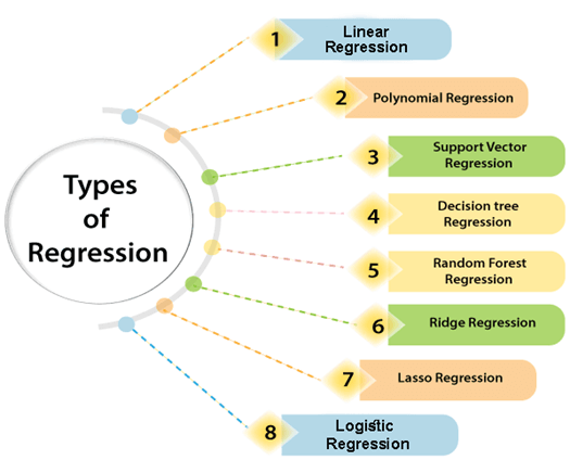
In addition to the nearest neighbor method, linear regression, and logistic regression, there are literally hundreds, if not thousands, of different machine learning techniques, but they all boil down to the same thing: trying to extract patterns and dependencies from data and using them either to gain understanding of a phenomenon or to predict future outcomes.

Machine learning can be a very hard problem and we can’t usually achieve a perfect method that would always produce the correct label. However, in most cases, a good but not perfect prediction is still better than none. Sometimes we may be able to produce better predictions by ourselves but we may still prefer to use machine learning because the machine will make its predictions faster and it will also keep churning out predictions without getting tired. Good examples are recommendation systems that need to predict what music, what videos, or what ads are more likely to be of interest to you.

The factors that affect how good a result we can achieve include:

• The hardness of the task: in handwritten digit recognition, if the digits are written very sloppily, even a human can’t always guess correctly what the writer intended
• The machine learning method: some methods are far better for a particular task than others
• The amount of training data: from only a few examples, it is impossible to obtain a good classifier
• The quality of the data

We know the importance of having enough data and the risks of over-fitting. Another equally important factor is the quality of the data. In order to build a model that generalises well to data outside of the training data, the training data needs to contain enough information that is relevant to the problem at hand. For example, if you create an image classifier that tells you what the image given to the algorithm is about, and you have trained it only on pictures of dogs and cats, it will assign everything it sees as either a dog or a cat. This would make sense if the algorithm is used in an environment where it will only see cats and dogs, but not if it is expected to see boats, cars, and flowers as well.

It is also important to emphasise that different machine learning methods are suitable for different tasks. Thus, there is no single best method for all problems (“one algorithm to rule them all...”). Fortunately, one can try out a large number of different methods and see which one of them works best in the problem at hand.

This leads us to a point that is very important but often overlooked in practice: what it means to work better. In the digit recognition task, a good method would of course produce the correct label most of the time. We can measure this by the classification error: the fraction of cases where our classifier outputs the wrong class. In predicting apartment prices, the quality measure is typically something like the difference between the predicted price and the final price for which the apartment is sold. In many real-life applications, it is also worse to err in one direction than in another: setting the price too high may delay the process by months, but setting the price too low will mean less money for the seller. And to take yet another example, failing to detect a pedestrian in front of a car is a far worse error than falsely detecting one when there is none.

We can’t usually achieve zero error, but perhaps we will be happy with error less than 1 in 100 (or 1%). This too depends on the application: you wouldn’t be happy to have only 99% safe cars on the streets, but being able to predict whether you’ll like a new song with that accuracy may be more than enough for a pleasant listening experience. Keeping the actual goal in mind at all times helps us make sure that we create actual added value.

Read More

Logistic regression

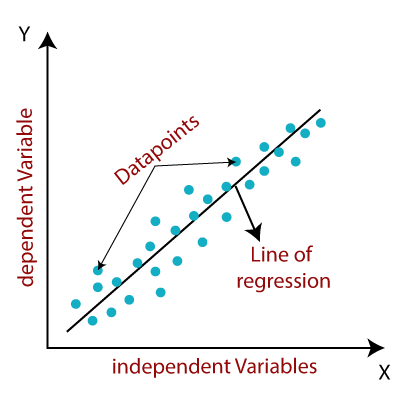
Linear regression is truly the workhorse of many AI and data science applications. It has its limits but they are often compensated by its simplicity, interpretability and efficiency. Linear regression has been successfully used in the following problems to give a few examples:

• prediction of click rates in online advertising
• prediction of retail demand for products
• prediction of box-office revenue of Hollywood movies
• prediction of software cost
• prediction of insurance cost
• prediction of crime rates
• prediction of real estate prices

Could we use regression to predict labels?

Linear regression and the nearest neighbor method produce different kinds of predictions. Linear regression outputs numerical outputs while the nearest neighbor method produces labels from a fixed set of alternatives (“classes”).

Where linear regression excels compared to nearest neighbors is interpretability. What do we mean by this? You could say that in a way, the nearest neighbor method and any single prediction that it produces are easy to interpret: it’s just the nearest training data element! This is true, but when it comes to the interpretability of the learned model, there is a clear difference. Interpreting the trained model in nearest neighbors in a similar fashion as the weights in linear regression is impossible: the learned model is basically the whole data, and it is usually way too big and complex to provide us with much insight. So what if we’d like to have a method that produces the same kind of outputs as the nearest neighbor, labels, but is interpretable like linear regression?

Logistic regression to the rescue

Well there is good news for you: we can turn the linear regression method’s outputs into predictions about labels. The technique for doing this is called logistic regression. We will not go into the technicalities, suffice to say that in the simplest case, we take the output from linear regression, which is a number, and predict one label A if the output is greater than zero, and another label B if the output is less than or equal to zero. Actually, instead of just predicting one class or another, logistic regression can also give us a measure of uncertainty of the prediction. So if we are predicting whether a customer will buy a new smartphone this year, we can get a prediction that customer A will buy a phone with probability 90%, but for another, less predictable customer, we can get a prediction that they will not buy a phone with 55% probability (or in other words, that they will buy one with 45% probability).

It is also possible to use the same trick to obtain predictions over more than two possible labels, so instead of always predicting either yes or no (buy a new phone or not, fake news or real news, and so forth), we can use logistic regression to identify, for example, handwritten digits, in which case there are ten possible labels.

An example of logistic regression

Let’s suppose that we collect data of students taking an introductory course in cookery. In addition to the basic information such as the student ID, name, and so on, we also ask the students to report how many hours they studied for the exam (however you study for a cookery exam, probably cooking?) – and hope that they are more or less honest in their reports. After the exam, we will know whether each student passed the course or not. Some data points are presented below:

Based on the table, what kind of conclusion could you draw between the hours studied and passing the exam? We could think that if we have data from hundreds of students, maybe we could see the amount needed to study in order to pass the course. We can present this data in a chart as you can see below.

Student ID	Hours studied	Pass/fail
24	15	Pass
41	9.5	Pass
58	2	Fail
101	5	Fail
103	6.5	Fail
215	6	Pass

Based on the table, what kind of conclusion could you draw between the hours studied and passing the exam? We could think that if we have data from hundreds of students, maybe we could see the amount needed to study in order to pass the course. We can present this data in a chart as you can see below:

 

Each dot on the figure corresponds to one student. On the bottom of the figure we have the scale for how many hours the student studied for the exam, and the students who passed the exam are shown as dots at the top of the chart, and the ones who failed are shown at the bottom. We´ll use the scale on the left to indicate the predicted probability of passing, which we´ll get from the logistic regression model as we explain just below. Based on this figure, you can see roughly that students who spent longer studying had better chances of passing the course. Especially the extreme cases are intuitive: with less than an hour’s work, it is very hard to pass the course, but with a lot of work, most will be successful. But what about those that spend time studying somewhere inbetween the extremes? If you study for 6 hours, what are your chances of passing?

We can quantify the probability of passing using logistic regression. The curve in the figure can be interpreted as the probability of passing: for example, after studying for five hours, the probability of passing is a little over 20%. We will not go into the details on how to obtain the curve, but it will be similar to how we learn the weights in linear regression.

If you wanted to have an 80% chance of passing a university exam, based on the above figure, how many hours should you approximately study for?

Your answer should be 10-11 hours.

Logistic regression is also used in a great variety of real-world AI applications such as predicting financial risks, in medical studies, and so on. However, like linear regression, it is also constrained by the linearity property and we need many other methods in our toolbox.

Read More