Creating a single layer neural network

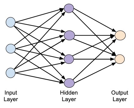
In this post, we are creating a single layer neural network that consists of independent neurons acting on input data to produce the output.

Note that we are using the text file named neural_simple.txt as our input.

Import the useful packages as shown:

import numpy as np
import matplotlib.pyplot as plt
import neurolab as nl

Load the dataset as follows:

input_data = np.loadtxt(“/Users/admin/neural_simple.txt')

The following is the data we are going to use. Note that in this data, first two columns are the features and last two columns are the labels.

array([[2. , 4. , 0. , 0. ],

[1.5, 3.9, 0. , 0. ],
[2.2, 4.1, 0. , 0. ],
[1.9, 4.7, 0. , 0. ],
[5.4, 2.2, 0. , 1. ],
[4.3, 7.1, 0. , 1. ],
[5.8, 4.9, 0. , 1. ],
[6.5, 3.2, 0. , 1. ],

[3. , 2. , 1. , 0. ],

[2.9, 0.3, 1. , 0. ],
[6.5, 8.3, 1. , 1. ],
[3.2, 6.2, 1. , 1. ],
[4.9, 7.8, 1. , 1. ],
[2.1, 4.8, 1. , 1. ]])

Now, separate these four columns into 2 data columns and 2 labels:

data = input_data[:, 0:2]
labels = input_data[:, 2:]

Plot the input data using the following commands:

plt.figure()
plt.scatter(data[:,0], data[:,1])
plt.xlabel('Dimension 1')
plt.ylabel('Dimension 2')
plt.title('Input data')

Now, define the minimum and maximum values for each dimension as shown here:

dim1_min, dim1_max = data[:,0].min(), data[:,0].max()
dim2_min, dim2_max = data[:,1].min(), data[:,1].max()

Next, define the number of neurons in the output layer as follows:

nn_output_layer = labels.shape[1]

Now, define a single-layer neural network:

dim1 = [dim1_min, dim1_max]
dim2 = [dim2_min, dim2_max]
neural_net = nl.net.newp([dim1, dim2], nn_output_layer)

Train the neural network with number of epochs and learning rate as shown:

error = neural_net.train(data, labels, epochs=200, show=20, lr=0.01)

Now, visualize and plot the training progress using the following commands:

plt.figure()
plt.plot(error)
plt.xlabel('Number of epochs')

plt.ylabel('Training error')
plt.title('Training error progress')
plt.grid()

plt.show()

Now, use the test data-points in above classifier:

print('\nTest Results:')

data_test = [[1.5, 3.2], [3.6, 1.7], [3.6, 5.7],[1.6, 3.9]] for item in data_test:
print(item, '-->', neural_net.sim([item])[0])

You can find the test results as shown here:

[1.5, 3.2] --> [1. 0.]

[3.6, 1.7] --> [1. 0.]
[3.6, 5.7] --> [1. 1.]

[1.6, 3.9] --> [1. 0.]

You can see the following graphs as the output of the code discussed till now:

In the next post we'll be creating a multi-layer neural network.