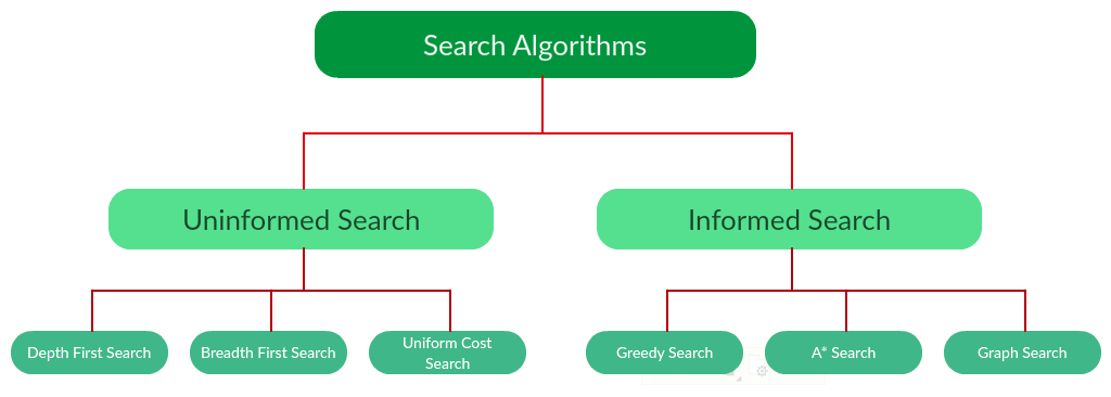
Heuristic Search in AI

Heuristic is a rule of thumb which leads us to the probable solution. Most problems in artificial intelligence are of exponential nature and have many possible solutions. You do not know exactly which solutions are correct and checking all the solutions would be very expensive.

Thus, the use of heuristic narrows down the search for solution and eliminates the wrong options. The method of using heuristic to lead the search in search space is called Heuristic Search. Heuristic techniques are very useful because the search can be boosted when you use them.

There are two types of control strategies or search techniques: uninformed and informed. They are explained in detail as given here:

Uninformed Search

It is also called blind search or blind control strategy. It is named so because there is information only about the problem definition, and no other extra information is available about the states. This kind of search techniques would search the whole state space for getting the solution. Breadth First Search (BFS) and Depth First Search (DFS) are the examples of uninformed search.

Informed Search

It is also called heuristic search or heuristic control strategy. It is named so because there is some extra information about the states. This extra information is useful to compute the preference among the child nodes to explore and expand. There would be a heuristic function associated with each node. Best First Search (BFS), A*, Mean and Analysis are the examples of informed search.

Constraint Satisfaction Problems (CSPs)

Constraint means restriction or limitation. In AI, constraint satisfaction problems are the problems which must be solved under some constraints. The focus must be on not to violate the constraint while solving such problems. Finally, when we reach the final solution, CSP must obey the restriction.

Now, let us apply this to real world problems too. Some examples of real world problems solved by constraint satisfaction are as follows:

1. Solving algebraic relation

With the help of constraint satisfaction problem, we can solve algebraic relations. In this example, we will try to solve a simple algebraic relation 𝒂∗𝟐 = 𝒃. It will return the value of 𝒂 and 𝒃 within the range that we would define.

After completing this Python program, you would be able to understand the basics of solving problems with constraint satisfaction.

Note that before writing the program, we need to install Python package called python-constraint. You can install it with the help of the following command:

pip install python-constraint

The following steps show you a Python program for solving algebraic relation using constraint satisfaction:

Import the constraint package using the following command:

from constraint import *

Now, create an object of module named problem() as shown below:

problem = Problem()

Now, define variables. Note that here we have two variables a and b, and we are defining 10 as their range, which means we got the solution within first 10 numbers.

problem.addVariable('a', range(10))
problem.addVariable('b', range(10))

Next, define the particular constraint that we want to apply on this problem. Observe that here we are using the constraint a*2 = b.

problem.addConstraint(lambda a, b: a * 2 == b)

Now, create the object of getSolution() module using the following command:

solutions = problem.getSolutions()

Lastly, print the output using the following command:

print (solutions)

You can observe the output of the above program as follows:

[{'a': 4, 'b': 8}, {'a': 3, 'b': 6}, {'a': 2, 'b': 4}, {'a': 1, 'b': 2}, {'a': 0, 'b': 0}]

2. Magic Square

A magic square is an arrangement of distinct numbers, generally integers, in a square grid, where the numbers in each row , and in each column , and the numbers in the diagonal, all add up to the same number called the “magic constant”.

The following is a stepwise execution of simple Python code for generating magic squares:

Define a function named magic_square, as shown below:

def magic_square(matrix_ms):
iSize = len(matrix_ms[0])
sum_list = []

The following code shows the code for vertical of squares:

for col in range(iSize):
sum_list.append(sum(row[col] for row in matrix_ms))

The following code shows the code for horizantal of squares:

sum_list.extend([sum (lines) for lines in matrix_ms])

The following code shows the code for horizontal of squares:

dlResult = 0

for i in range(0,iSize):
     dlResult +=matrix_ms[i][i]
sum_list.append(dlResult)
drResult = 0
for i in range(iSize-1,-1,-1):
    drResult +=matrix_ms[i][i]
sum_list.append(drResult)

if len(set(sum_list))>1:
    return False
return True

Now, give the value of the matrix and check the output:

print(magic_square([[1,2,3], [4,5,6], [7,8,9]]))

You can observe that the output would be False as the sum is not up to the same number.

print(magic_square([[3,9,2], [3,5,7], [9,1,6]]))

You can observe that the output would be True as the sum is the same number, that is 15 here.