Analyzing Sequential Data by Hidden Markov Model (HMM)

HMM is a statistic model which is widely used for data having continuation and extensibility such as time series stock market analysis, health checkup, and speech recognition. This post deals in detail with analyzing sequential data using Hidden Markov Model (HMM).

Hidden Markov Model (HMM)

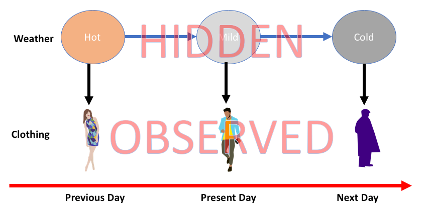
HMM is a stochastic model which is built upon the concept of Markov chain based on the assumption that probability of future stats depends only on the current process state rather any state that preceded it. For example, when tossing a coin, we cannot say that the result of the fifth toss will be a head. This is because a coin does not have any memory and the next result does not depend on the previous result.

Mathematically, HMM consists of the following variables:

States (S)

It is a set of hidden or latent states present in a HMM. It is denoted by S.

Output symbols (O)

It is a set of possible output symbols present in a HMM. It is denoted by O.

State Transition Probability Matrix (A)

It is the probability of making transition from one state to each of the other states. It is denoted by A.

Observation Emission Probability Matrix (B)

It is the probability of emitting/observing a symbol at a particular state. It is denoted by B.

Prior Probability Matrix (Π)

It is the probability of starting at a particular state from various states of the system. It is denoted by Π.

Hence, a HMM may be defined as 𝝀=(𝑺,𝑶,𝑨,𝑩,𝝅),

where, 𝑺={𝒔𝟏,𝒔𝟐,…,𝒔𝑵} is a set of N possible states,
𝑶={𝒐𝟏,𝒐𝟐,…,𝒐𝑴} is a set of M possible observation symbols,
A is an 𝑵𝒙𝑵 state Transition Probability Matrix (TPM),
B is an 𝑵𝒙𝑴 observation or Emission Probability Matrix (EPM),
π is an N dimensional initial state probability distribution vector.

Now we are going to analyze the data of stock market, step by step, to get an idea about how the HMM works with sequential or time series data. Please note that we are implementing this example in Python.
Import the necessary packages as shown below:

import datetime
import warnings

Now, use the stock market data from the matpotlib.finance package, as shown here:

import numpy as np
from matplotlib import cm, pyplot as plt
from matplotlib.dates import YearLocator, MonthLocator
try:
from matplotlib.finance import quotes_historical_yahoo_och1
except ImportError:
from matplotlib.finance import (
quotes_historical_yahoo as quotes_historical_yahoo_och1)
from hmmlearn.hmm import GaussianHMM

Load the data from a start date and end date, i.e., between two specific dates as shown here:

start_date = datetime.date(1995, 10, 10)
end_date = datetime.date(2015, 4, 25)
quotes = quotes_historical_yahoo_och1('INTC', start_date, end_date)

In this step, we will extract the closing quotes every day. For this, use the following command:

closing_quotes = np.array([quote[2] for quote in quotes])

Now, we will extract the volume of shares traded every day. For this, use the following command:

volumes = np.array([quote[5] for quote in quotes])[1:]

Here, take the percentage difference of closing stock prices, using the code shown below:

diff_percentages = 100.0 * np.diff(closing_quotes) / closing_quotes[:-]
dates = np.array([quote[0] for quote in quotes], dtype=np.int)[1:]
training_data = np.column_stack([diff_percentages, volumes])

In this step, create and train the Gaussian HMM. For this, use the following code:

hmm = GaussianHMM(n_components=7, covariance_type='diag', n_iter=1000)
with warnings.catch_warnings():
warnings.simplefilter('ignore')
hmm.fit(training_data)

Now, generate data using the HMM model, using the commands shown:

num_samples = 300
samples, _ = hmm.sample(num_samples)

Finally, in this step, we plot and visualize the difference percentage and volume of shares traded as output in the form of graph.

Use the following code to plot and visualize the difference percentages:

plt.figure()
plt.title('Difference percentages')
plt.plot(np.arange(num_samples), samples[:, 0], c='black')

Use the following code to plot and visualize the volume of shares traded:

plt.figure()
plt.title('Volume of shares')
plt.plot(np.arange(num_samples), samples[:, 1], c='black')
plt.ylim(ymin=0)

plt.show()

This is the end of today's post. In the next post, we will learn about speech recognition using AI with Python.