Using MatPlotLib to graph the loss and the accuracy for ML algorithms

In this post we are going to run our base code from the previous post again and do some analysis of the run using MatPlotLib. Assuming MatPlotLib is installed (if not pip3 install MatPlotLib) we'll do the following changes to the code from previous post:

1. Add the history variable to the output of the model.fit to collect data.
2. Add MatPlotLib commands to graph the loss and the accuracy from our epochs.
3. Add figure displays for our two individual image tests.

The following program incorporates the above mentioned changes:

#import libraries
import numpy as np
import matplotlib.pyplot as plt
import matplotlib.image as mpimg
import seaborn as sns
import tensorflow as tf
from tensorflow.python.framework import ops
from tensorflow.examples.tutorials.mnist import input_data
from PIL import Image
# Import Fashion MNIST
fashion_mnist = input_data.read_data_sets('input/data', one_hot=True)
fashion_mnist = tf.keras.datasets.fashion_mnist
(train_images, train_labels), (test_images, test_labels) = fashion_mnist.
load_data()
class_names = ['T-shirt/top', 'Trouser', 'Pullover', 'Dress', 'Coat',
'Sandal', 'Shirt', 'Sneaker', 'Bag', 'Ankle boot']
train_images = train_images / 255.0
test_images = test_images / 255.0
model = tf.keras.Sequential()
model.add(tf.keras.layers.Flatten(input_shape=(28,28)))
model.add(tf.keras.layers.Dense(128, activation='relu' ))
model.add(tf.keras.layers.Dense(10, activation='softmax' ))
model.compile(optimizer=tf.train.AdamOptimizer(),
loss='sparse_categorical_crossentropy',
metrics=['accuracy'])
history = model.fit(train_images, train_labels, epochs=2) 
# Get training and test loss histories
training_loss = history.history['loss']
accuracy = history.history['acc']
# Create count of the number of epochs
epoch_count = range(1, len(training_loss) + 1)
# Visualize loss history
plt.figure(0)
plt.plot(epoch_count, training_loss, 'r--')
plt.plot(epoch_count, accuracy, 'b--')
plt.legend(['Training Loss', 'Accuracy'])
plt.xlabel('Epoch')
plt.ylabel('History')
plt.show(block=False);
plt.pause(0.001)
test_loss, test_acc = model.evaluate(test_images, test_labels)
#run test image from Fashion_MNIST data
img = test_images[15]
plt.figure(1)
plt.imshow(img)
plt.show(block=False)
plt.pause(0.001)
img = (np.expand_dims(img,0))
singlePrediction = model.predict(img,steps=1)
print ("Prediction Output")
print(singlePrediction)
print()
NumberElement = singlePrediction.argmax()
Element = np.amax(singlePrediction)
print ("Our Network has concluded that the image number '15' is a "
+class_names[NumberElement])
print (str(int(Element*100)) + "% Confidence Level")
print('Test accuracy:', test_acc)
# read test dress image
imageName = "Dress28x28.JPG"
testImg = Image.open(imageName)
plt.figure(2)
plt.imshow(testImg)
plt.show(block=False)
plt.pause(0.001)
testImg.load()
data = np.asarray( testImg, dtype="float" )
data = tf.image.rgb_to_grayscale(data)
data = data/255.0
data = tf.transpose(data, perm=[2,0,1])
singlePrediction = model.predict(data,steps=1)
NumberElement = singlePrediction.argmax()
Element = np.amax(singlePrediction)
print(NumberElement)
print(Element)
print(singlePrediction)
print ("Our Network has concluded that the file '"+imageName+"' is a
"+class_names[NumberElement])
print (str(int(Element*100)) + "% Confidence Level")
plt.show()

When we run this program the following plots are obtained:

Figure 0

 Figure 1

  Figure 2

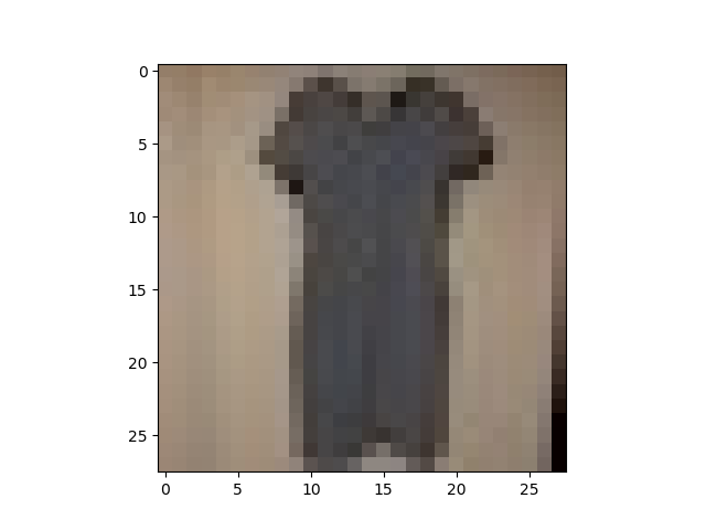
The window labeled Figure 0 shows the accuracy data for each of the five epochs of the machine learning training, and you can see the accuracy slowly increases with each epoch. The window labeled Figure 1 shows the test picture used for the first recognition test (it found a pair of trousers, which is correct), and finally, the window labeled Figure 2 shows the dress picture, which is still incorrectly identified as a bag and our output window shows this:

10000/10000 [==============================] - 0s 43us/sample - loss: 0.3492 - a
cc: 0.8756
Prediction Output
[[4.1143132e-05 9.9862289e-01 6.8796166e-06 1.1105506e-03 2.1581816e-04
  8.0114615e-10 2.3793352e-06 3.6482924e-11 2.4894479e-07 3.7706857e-10]]

Our Network has concluded that the image number '15' is a Trouser
99% Confidence Level
Test accuracy: 0.8756
8
0.9999794
[[2.7322454e-07 4.4263427e-08 2.3696880e-07 1.3007481e-08 5.6515717e-08
  3.5395464e-11 1.9993138e-05 1.4521572e-13 9.9997938e-01 5.2564192e-13]]
Our Network has concluded that the file 'Dress28x28.JPG' is a Bag
99% Confidence Level
------------------
(program exited with code: 0)

Press any key to continue . . .

Here I am ending this post. Hope you begin to understand the theory behind a lot of the models we have use, you should now have the ability to build and experiment with making machines learn. See you soon with a new topic, till then keep practicing and learning Python as Python is easy to learn!