Pandas - 52 Develop neural networks with TensorFlow - Test Phase and Accuracy Calculation

After having an educated neural network, we can create the evaluations and calculate the accuracy. First we define a testing set with elements different than the training set. For convenience, these examples always use 11 elements. See the following program:

import tensorflow as tf
import numpy as np
import matplotlib.pyplot as plt

#Testing set

testX = np.array([[1.,2.25],[1.25,3.],[2,2.5],[2.25,2.75],[2.5,3.],[2.,0.9],[2.5,1.2],[3.,1.25],[3.,1.5],[3.5,2.],[3.5,2.5]])
testY = [[1.,0.]]*5 + [[0.,1.]]*6
print('\ntestX\n')
print(testX)
print('\ntestY\n')
print(testY)

The output of the program is shown below:

testX

[[1.   2.25]
 [1.25 3.  ]
 [2.   2.5 ]
 [2.25 2.75]
 [2.5  3.  ]
 [2.   0.9 ]
 [2.5  1.2 ]
 [3.   1.25]
 [3.   1.5 ]
 [3.5  2.  ]
 [3.5  2.5 ]]

testY

[[1.0, 0.0], [1.0, 0.0], [1.0, 0.0], [1.0, 0.0], [1.0, 0.0], [0.0, 1.0], [0.0, 1
.0], [0.0, 1.0], [0.0, 1.0], [0.0, 1.0], [0.0, 1.0]]
------------------
(program exited with code: 0)

Press any key to continue . . .

As a standard practice it's better to test data set points on a chart:

yc = [0]*5 + [1]*6
print('\nyc\n')
print(yc)
plt.scatter(testX[:,0],testX[:,1],c=yc, s=50, alpha=0.9)
plt.show()

Add the code shown above in the previous program and it should generate the following output:

yc

[0, 0, 0, 0, 0, 1, 1, 1, 1, 1, 1]

As our testing set is ready we can use it to evaluate the SLP neural network and calculate the accuracy. See the following code:

init = tf.global_variables_initializer()
with tf.Session() as sess:
   
    sess.run(init)
    for i in range(training_epochs):
        sess.run(optimizer, feed_dict = {x: inputX, y: inputY})
    pred = tf.nn.softmax(evidence)   
    result = sess.run(pred, feed_dict = {x: testX})
    correct_prediction = tf.equal(tf.argmax(pred, 1),tf.argmax(testY, 1))
   
    # Calculate accuracy
   
    accuracy = tf.reduce_mean(tf.cast(correct_prediction, "float"))
    print("Accuracy:", accuracy.eval({x: testX, y: testY}))
   
yc = result[:,1]
plt.scatter(testX[:,0],testX[:,1],c=yc, s=50, alpha=1)
plt.show()

The output of the program is shown below:

testX

[[1.   2.25]
 [1.25 3.  ]
 [2.   2.5 ]
 [2.25 2.75]
 [2.5  3.  ]
 [2.   0.9 ]
 [2.5  1.2 ]
 [3.   1.25]
 [3.   1.5 ]
 [3.5  2.  ]
 [3.5  2.5 ]]

testY

[[1.0, 0.0], [1.0, 0.0], [1.0, 0.0], [1.0, 0.0], [1.0, 0.0], [0.0, 1.0], [0.0, 1
.0], [0.0, 1.0], [0.0, 1.0], [0.0, 1.0], [0.0, 1.0]]

yc

[0, 0, 0, 0, 0, 1, 1, 1, 1, 1, 1]
Accuracy: 1.0
------------------
(program exited with code: 0)

Press any key to continue . . .

From the output we can see that the neural network was able to correctly classify all 11 past champions. It displays the points on the Cartesian plane with the same system of color gradations
ranging from dark blue to yellow as shown in the graph below:

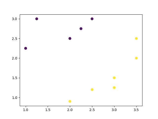The results can be considered optimal, given the simplicity of the model used and the small amount of data used in the training set.

Here I am ending today's discussion wherein we learned Test Phase and Accuracy Calculation. In the next post I'll focus on Multi Layer Perceptron with TensorFlow . So till we meet again keep learning and practicing Python as Python is easy to learn!