Neural networks are good models for how brains learn and classify data. Given that, it is no surprise that neural networks show up in machine learning and other AI techniques. A neural network consists of the following parts:
When we set up a network of neurons (and we do define the architecture and layout — creating an arbitrary network of connections has turned into what we call “evolutionary computing”) one of the most important choices we make is the activation function (sometimes known as the threshold for the
neuron to fire). This activation function is one of the key things we define when we build our Python models of neurons.
Let's first discuss about a two layer neural network which actually consists of three layers but the input layer is typically excluded when we count a neural network’s layers. See the diagram below:
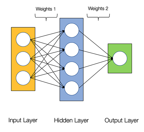
By looking at this diagram, we can see that the neurons on each layer are connected to all the neurons of the next layer. Weights are given for each of the inter-neural connecting lines.
A neuron, as the word is used in AI, is a software model of a nervous system cell that behaves more or less like an actual brain neuron. The model uses numbers to make one neuron or another be more important to the results. These numbers are called weights.
The figure also shows the input layer, the hidden layer (so called because it is not directly connected to the outside world), and the output layer. This is a very simple network; real networks are much more complex with multiple more layers. In fact, deep learning gets its name from the fact that you have multiple hidden layers, in a sense increasing the “depth” of the neural network.
We have the layers filter and process information from left to right in a progressive fashion. This is called a feed-forward input because the data feeds in only one direction.
So, now that we have a network, the next question that comes to our mind is, how does it learn?
The neuron network receives an example and guesses at the answer (by using whatever default weights and biases that they start with). If the answer is wrong, it backtracks and modifies the weights and biases in the neurons and tries to fix the error by changing some values. This is called back-propagation and simulates what people do when performing a task using an iterative approach for trial and error. See the figure below:

After we repeat this process many times, eventually the neural network begins to get better (learns) and provides better answers. Each one of these iterations is called an epoch. This name fits pretty well because sometimes it can take days or weeks to provide training to learn complex tasks.
Although it may take days or weeks to train a neural net, after it is trained, we can duplicate it with little effort by copying the topology, weights, and biases of the trained network. When we have a trained neural net, we can use it easily again and again, until we need something different. Then, it is back to training.
Neural networks, as such, do model some types of human learning. However, humans have significantly more complex ways available for hierarchically categorizing objects (such as categorizing horses and pigs as animals) with little effort. Neural networks (and the whole deep learning field) are not very good at transferring knowledge and results from one type of situation to another without retraining.
Looking at the network in Figure shown above, we can see that the output of this neural networks is only dependent on the weights of the interconnection and also something we call the biases of the neurons themselves. Although the weights affect the steepness of the activation function curve (more on that later), the bias will shift the entire curve to the right or left. The choices of the weights and biases determines the strength of predictions of the individual neurons. Training the neural network involves using the input data to fine-tune the weights and biases.
The activation function
An activation function is a key part of our neuron model. This is the software function that determines whether information passes through or is stopped by the individual neuron. However, we don’t just use it as a gate (open or shut), we use it as a function that transforms the input signal to the neuron in some useful way.
There are many types of activation functions available. For our simple neural network, we will use one of the most popular ones — the sigmoid function. A sigmoid function has a characteristic “S” curve, as shown in Figure below:
 If we apply a 1.0 value bias to the curve in Figure shown above, then the whole curve shifts to the right, making the (0,0.5) point move to (1,0.5).
Loss function
The loss function compares the result of our neural network to the desired results. Another way of thinking of this is that the loss function tells us how good our current results are. This is the information that we are looking for to supply it to our back-propagation channel that will improve our neural network.
Later we'll use a function that finds the derivative of the loss function towards our result (the slope of the curve is the first derivative calculus fans) to figure out what to do with our neuron weights. This is a major part of the “learning” activity of the network.
In this post we have discussed about all the parts of our neural network, in the next post we'll build an
example. So until we meet again keep practicing and learning Python as Python is easy to learn!
- The input layer of neurons
- An arbitrary amount of hidden layers of neurons
- An output layer of neurons connecting to the world
- A set of weights and biases between each neuron level
- A choice of activation function for each hidden layer of neurons
- A loss function that will provide “overtraining” of the network
When we set up a network of neurons (and we do define the architecture and layout — creating an arbitrary network of connections has turned into what we call “evolutionary computing”) one of the most important choices we make is the activation function (sometimes known as the threshold for the
neuron to fire). This activation function is one of the key things we define when we build our Python models of neurons.
Let's first discuss about a two layer neural network which actually consists of three layers but the input layer is typically excluded when we count a neural network’s layers. See the diagram below:
By looking at this diagram, we can see that the neurons on each layer are connected to all the neurons of the next layer. Weights are given for each of the inter-neural connecting lines.
A neuron, as the word is used in AI, is a software model of a nervous system cell that behaves more or less like an actual brain neuron. The model uses numbers to make one neuron or another be more important to the results. These numbers are called weights.
The figure also shows the input layer, the hidden layer (so called because it is not directly connected to the outside world), and the output layer. This is a very simple network; real networks are much more complex with multiple more layers. In fact, deep learning gets its name from the fact that you have multiple hidden layers, in a sense increasing the “depth” of the neural network.
We have the layers filter and process information from left to right in a progressive fashion. This is called a feed-forward input because the data feeds in only one direction.
So, now that we have a network, the next question that comes to our mind is, how does it learn?
The neuron network receives an example and guesses at the answer (by using whatever default weights and biases that they start with). If the answer is wrong, it backtracks and modifies the weights and biases in the neurons and tries to fix the error by changing some values. This is called back-propagation and simulates what people do when performing a task using an iterative approach for trial and error. See the figure below:

After we repeat this process many times, eventually the neural network begins to get better (learns) and provides better answers. Each one of these iterations is called an epoch. This name fits pretty well because sometimes it can take days or weeks to provide training to learn complex tasks.
Although it may take days or weeks to train a neural net, after it is trained, we can duplicate it with little effort by copying the topology, weights, and biases of the trained network. When we have a trained neural net, we can use it easily again and again, until we need something different. Then, it is back to training.
Neural networks, as such, do model some types of human learning. However, humans have significantly more complex ways available for hierarchically categorizing objects (such as categorizing horses and pigs as animals) with little effort. Neural networks (and the whole deep learning field) are not very good at transferring knowledge and results from one type of situation to another without retraining.
Looking at the network in Figure shown above, we can see that the output of this neural networks is only dependent on the weights of the interconnection and also something we call the biases of the neurons themselves. Although the weights affect the steepness of the activation function curve (more on that later), the bias will shift the entire curve to the right or left. The choices of the weights and biases determines the strength of predictions of the individual neurons. Training the neural network involves using the input data to fine-tune the weights and biases.
The activation function
An activation function is a key part of our neuron model. This is the software function that determines whether information passes through or is stopped by the individual neuron. However, we don’t just use it as a gate (open or shut), we use it as a function that transforms the input signal to the neuron in some useful way.
There are many types of activation functions available. For our simple neural network, we will use one of the most popular ones — the sigmoid function. A sigmoid function has a characteristic “S” curve, as shown in Figure below:

Loss function
The loss function compares the result of our neural network to the desired results. Another way of thinking of this is that the loss function tells us how good our current results are. This is the information that we are looking for to supply it to our back-propagation channel that will improve our neural network.
Later we'll use a function that finds the derivative of the loss function towards our result (the slope of the curve is the first derivative calculus fans) to figure out what to do with our neuron weights. This is a major part of the “learning” activity of the network.
In this post we have discussed about all the parts of our neural network, in the next post we'll build an
example. So until we meet again keep practicing and learning Python as Python is easy to learn!
0 comments:
Post a Comment