Friday, January 6, 2023

Linear Regression

It is used to estimate real values (cost of houses, number of calls, total sales etc.) based on continuous variable(s). Here, we establish the relationship between independent and dependent variables by fitting the best line. This best fit line is known as the regression line and is represented by a linear equation Y= a *X + b.

The best way to understand linear regression is to relive this experience of childhood. Let us say, you ask a child in fifth grade to arrange people in his class by increasing the order of weight, without asking them their weights! What do you think the child will do? He/she would likely look (visually analyze) at the height and build of people and arrange them using a combination of these visible parameters. This is linear regression in real life! The child has actually figured out that height and build would be correlated to weight by a relationship, which looks like the equation above.

In this equation:

  • Y – Dependent Variable
  • a – Slope
  • X – Independent variable
  • b – Intercept

These coefficients a and b are derived based on minimizing the sum of the squared difference of distance between data points and the regression line.

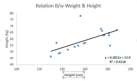
Look at the below example. Here we have identified the best fit line having linear equation y=0.2811x+13.9. Now using this equation, we can find the weight, knowing the height of a person.
Linear_Regression | machine learning algorithms

Linear Regression is mainly of two types: Simple Linear Regression and Multiple Linear Regression. Simple Linear Regression is characterized by one independent variable. And, Multiple Linear Regression(as the name suggests) is characterized by multiple (more than 1) independent variables. While finding the best fit line, you can fit a polynomial or curvilinear regression. And these are known as polynomial or curvilinear regression. 

Share:

MongoDB

MongoDB is an unstructured database. It stores data in the form of documents. MongoDB is able to handle huge volumes of data very efficiently and is the most widely used NoSQL database as it offers rich query language and flexible and fast access to data.

Let’s take a moment to understand the architecture of a MongoDB database.

The Architecture of a MongoDB Database

The information in MongoDB is stored in documents. Here, a document is analogous to rows in structured databases.

  • Each document is a collection of key-value pairs
  • Each key-value pair is called a field
  • Every document has an _id  field, which uniquely identifies the documents
  • A document may also contain nested documents
  • Documents may have a varying number of fields (they can be blank as well)

These documents are stored in a collection. A collection is literally a collection of documents in MongoDB. This is analogous to tables in traditional databases.

Unlike traditional databases, the data is generally stored in a single collection in MongoDB, so there is no concept of joins (except $lookup operator, which performs left-outer-join like operation). MongoDB has the nested document instead. 

Share:

Wednesday, January 4, 2023

Machine Learning Algorithms


1. Supervised Learning Algorithms

How it works: This algorithm consists of a target/outcome variable (or dependent variable) which is to be predicted from a given set of predictors (independent variables). Using this set of variables, we generate a function that map inputs to desired outputs. The training process continues until the model achieves a desired level of accuracy on the training data. Examples of Supervised Learning: Regression, Decision Tree, Random Forest , KNN, Logistic Regression etc.


2. Unsupervised Learning Algorithms

How it works: In this algorithm, we do not have any target or outcome variable to predict / estimate. It is used for clustering populations in different groups, which is widely used for segmenting customers into different groups for specific interventions. Examples of Unsupervised Learning: Apriori algorithm, K-means.


3. Reinforcement Learning:

How it works: Using this algorithm, the machine is trained to make specific decisions. It works this way: the machine is exposed to an environment where it trains itself continually using trial and error. This machine learns from past experience and tries to capture the best possible knowledge to make accurate business decisions. Example of Reinforcement Learning: Markov Decision Process

Here is the list of commonly used machine learning algorithms. These algorithms can be applied to almost any data problem:

  1. Linear Regression
  2. Logistic Regression
  3. Decision Tree
  4. SVM
  5. Naive Bayes
  6. kNN
  7. K-Means
  8. Random Forest
  9. Dimensionality Reduction Algorithms
  10. Gradient Boosting algorithms
    1. GBM
    2. XGBoost
    3. LightGBM
    4. CatBoost
Share:

Monday, January 2, 2023

Components of a Time Series Forecasting in Python

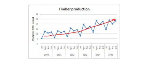
 1. Trend: A trend is a general direction in which something is developing or changing. So we see an increasing trend in this time series. We can see that the passenger count is increasing with the number of years. Let’s visualize the trend of a time series:


Trend

Example

Here the red line represents an increasing trend of the time series.

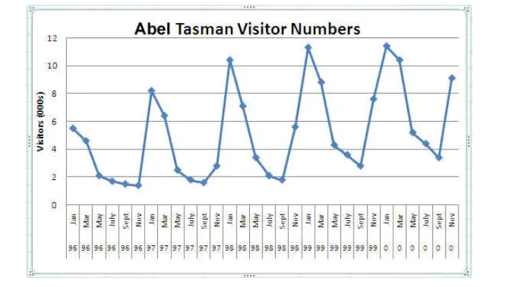
2. Seasonality:–  Another clear pattern can also be seen in the above time series, i.e., the pattern is repeating at a regular time interval which is known as the seasonality. Any predictable change or pattern in a time series that recurs or repeats over a specific time period can be said to be seasonality. Let’s visualize the seasonality of the time series:

Seasonality


Example

We can see that the time series is repeating its pattern after every 12 months i.e there is a peak every year during the month of January and a trough every year in the month of September, hence this time series has a seasonality of 12 months.

Difference Between a Time Series and Regression Problem

Here you might think that as the target variable is numerical it can be predicted using regression techniques, but a time series problem is different from a regression problem in the following ways:

  • The main difference is that a time series is time-dependent. So the basic assumption of a linear regression model that the observations are independent doesn’t hold in this case.
  • Along with an increasing or decreasing trend, most Time Series have some form of seasonality trends,i.e. variations specific to a particular time frame.


So, predicting a time series using regression techniques is not a good approach.

Time series analysis comprises methods for analyzing time-series data in order to extract meaningful statistics and other characteristics of the data. Time series forecasting is the use of a model to predict future values based on previously observed values.

Share:

Thursday, December 29, 2022

Time Series Data

Which of the following do you think is an example of time series? Even if you don’t know, try making a guess.


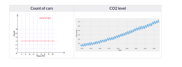
Time Series is generally data that is collected over time and is dependent on it. Here we see that the count of cars is independent of time, hence it is not a time series. While the CO2 level increases with respect to time, hence it is a time series.

Let us now look at the formal definition of Time Series.

This article was published as a part of the Data Science Blogathon.

Introduction on Time Series Forecasting Python

Unicorn Investors wants to make an investment in a new form of transportation – JetRail. JetRail uses Jet propulsion technology to run rails and move people at a high speed! The investment would only make sense if they can get more than 1 Million monthly users within the next 18 months. In order to help Unicorn Ventures in their decision, you need to forecast the traffic on JetRail for the next 7 months. You are provided with traffic data of JetRail since inception in the test file.

You can get the dataset here 

It is advised to look at the dataset after completing the hypothesis generation part.

Let’s Understand, What is Time Series Data?

Which of the following do you think is an example of time series? Even if you don’t know, try making a guess.

Time Series Data

Time Series is generally data that is collected over time and is dependent on it. Here we see that the count of cars is independent of time, hence it is not a time series. While the CO2 level increases with respect to time, hence it is a time series.

Let us now look at the formal definition of Time Series.

A series of data points collected in time order is known as a time series. Most business houses work on time series data to analyze sales numbers for the next year, website traffic, count of traffic, the number of calls received, etc. Data of a time series can be used for forecasting.

Not every data collected with respect to time represents a time series. Some of the examples of time series prediction Python are:

Stock Price


Passenger Count of Airlines


Temperature Over Time


A Number of Visitors in a Hotel

Now that we can differentiate between a Time Series and a non-Time Series data. let us explore Time Series further.

Now as we have an understanding of what a time series is and the difference between a time series and a non-time series, let’s look at the components of a time series in the next post.


Share:

Friday, December 9, 2022

What are datetimes?

You probably already understand that in the computer memory, all numeric information is represented as ones and zeros, so at the most basic level, there isn't anything special about dates or times. However, when working with real data in business and technical projects, we tend to think about time or dates in their own units, differently from other numbers. Time is most often thought of as hours, minutes, or seconds, and dates are usually years, months, and days. Other common patterns are the weekdays, day of the week, business days, and quarters. We often group data into bins of days, weeks, months, or quarters. Within these bins, there might be data every second, minute, hour, or on some other or even random period. Because it is natural to think of dates and time of day together, Python in general, and pandas in particular, provides objects to make it easy to work this way. The most fundamental time component in pandas is Timestamp, and it is equivalent to Datetime in Python, provided by the datetime package. Timestamp is used as the index for pandas time series data types, as we'll see a bit later. pandas provides the Timestamp method to convert various types of data into timestamps. Here, we convert a string in a familiar date format into a pandas timestamp:

my_timestamp = pd.Timestamp('12-25-2020')

my_timestamp

This code snippet produces the following output:


It's intuitive that Timestamp consists of year, month, day, hour, minute, and second. Since we did not provide any time information, Timestamp() assumes that the time portion is 00:00:00. The fact that Timestamp has these components is what makes pandas times series operations so flexible. To illustrate that pandas is already simplifying things for us, here, we import Python datetime, and use it to accomplish the same conversion:

from datetime import datetime

my_datetime = datetime.strptime('12-25-2020','%m-%d-%Y')

my_datetime

This produces the following output:


You can see that, in the case of using the datetime method, we have to provide a date format for Python to decode the string. The two resulting objects have very similar methods available to them.

Share:

Tuesday, December 6, 2022

Time series data

Time series data is nearly ubiquitous but can be a pain point in many analyses. For example, suppose you are asked to forecast sales for a retail store and are given daily sales figures for the last 6 months. When you review the data, you realize the store is usually open 5 days a week but sometimes has sales on Saturdays and even some Sundays. This makes most weekend days have missing values, and the time interval of the data is inconsistent. Also, when you consider estimating a monthly forecast, you realize months are of different lengths and have varying numbers of sales days. As simple and obvious as the issues are, they create a number of issues in analyzing and modeling the data over time.

The machine learning literature and popular articles are heavily biased toward classification problems, with little mention of time series. Yet much of the data we deal with is time series or at least starts out that way. Time series is a general term used to refer to data that is naturally ordered by time. For example, tweets arrive as a stream of timestamped data. Similarly, store transactions or online credit card transactions are time series. The log streams from data centers are time series.

It's important to note that, unlike tabular data in classification problems, time series data is ordered. In tabular data, random samples are shuffled before being used in a model. In time series, the order matters and we generally want to preserve it. The temporal relationship of events is critical; we can only recognize unusual server traffic if we analyze the sequence of data compared to normal use periods. The time sequence of store transactions can be compared day to day and over longer periods to anticipate high demand periods for inventory and staff planning. The examples are endless.

pandas has a wide range of features to work with time series data. In the pandas documentation, it is noted that pandas time series objects are based on NumPy datetime64 and timedelta64 object types. pandas consolidates some useful methods from libraries such as scikit.timeseries (so much so that pandas will eventually absorb this library), and adds a lot of additional functionality used for working with time series data. In this chapter, we'll introduce some of the more important capabilities and review how to deal with timestamps in data. The key to understanding how time series differs from other pandas data structures is that pandas provides a couple of additional object types, namely Timestamp and Timedelta, as well as Period.

Share:

Thursday, December 1, 2022

Components and applications of pandas

The pandas library is comprised of the following components:

• pandas/core: This contains the implementations of the basic data structures of pandas, such as Series and DataFrames. Series and DataFrames are basic toolsets that are very handy for data manipulation and are used extensively by data scientists.

• pandas/src: This consists of algorithms that provide the basic functionalities of pandas. These functionalities are part of the architecture of pandas, which you will not be using explicitly. This layer is written in C or Cython.

• pandas/io: This comprises toolsets for the input and output of files and data. These toolsets facilitate data input from sources such as CSV and text and allow you to write data to formats such as text and CSV.

• pandas/tools: This layer contains all the code and algorithms for pandas functions and methods, such as merge, join, and concat.

• pandas/sparse: This contains the functionalities for handling missing values within its data structures, such as DataFrames and Series.

• pandas/stats: This contains a set of tools for handling statistical functions such as regression and classification.

• pandas/util: This contains all the utilities for debugging the library.

• pandas/rpy: This is the interface for connecting to R.

The versatility of its different architectural components makes pandas useful in many real-world applications. Various data-wrangling functionalities in pandas (such as merge, join, and concatenation) save time when building real-world applications. Some notable applications where the pandas library can come in handy are as follows:

• Recommendation systems

• Advertising

• Stock predictions

• Neuroscience

• Natural language processing (NLP)

The list goes on. What's more important to note is that these are applications that have an impact on people's daily lives. For this reason, learning pandas has the potential to give a fillip to your analytics career.


Share:

Monday, November 21, 2022

pandas DataFrames

A pandas DataFrame is a 2D labeled data structure with columns that can be of different types. A DataFrame can be thought of as a dictionary-like container for Series objects, where each key in the dictionary is a column label and each value is a Series.

If you are familiar with relational databases, you’ll notice that a pandas DataFrame is similar to a regular SQL table. The figure below illustrates an

example of a pandas DataFrame.


Notice that the DataFrame includes an index column. Like with Series, pandas uses zero-based numeric indexing for DataFrames by default.

However, you can replace the default index with one or more existing columns. Figure below shows the same DataFrame but with the Date column set as the index.


In this particular example, the index is a column of type date. In fact, pandas allows you to have DataFrame indexes of any type. The most commonly used index types are integers and strings. However, you are not limited to using only simple types. You might define an index of a sequence type, such as List or Tuple, or even use an object type that is not built into Python; this could be a third-party type or even your own object type.

Share:

Thursday, November 17, 2022

Combining Series into a DataFrame

Multiple Series can be combined to form a DataFrame. Let’s try this by creating another Series and combining it with the emps_names Series: 

data = ['jeff.russell','jane.boorman','tom.heints']

emps_emails = pd.Series(data,index=[9001,9002,9003], name ='emails')

emps_names.name = 'names'

df = pd.concat([emps_names,emps_emails], axis=1)

print(df)

To create the new Series, you call the Series() constructor , passing the following arguments: the list to be converted to a Series, the indices of the Series, and the name of the Series.

You need to name Series before concatenating them into a DataFrame, because their names will become the names of the corresponding DataFrame columns. Since you didn’t name the emps_names Series when you created it earlier, you name it here by setting its name property to 'names'. After that, you can concatenate it with the emps_emails Series. You specify axis=1 in order to concatenate along the columns.

The resulting DataFrame looks like this:

names     emails

9001        Jeff Russell jeff.russell

9002        Jane Boorman jane.boorman

9003        Tom Heints tom.heints

Share:

Monday, November 14, 2022

Accessing Data in a Series

To access an element in a Series, specify the Series name followed by the element’s index within square brackets, as shown here:

print(emps_names[9001])

This outputs the element corresponding to index 9001:

Jeff Russell

Alternatively, you can use the loc property of the Series object:

print(emps_names.loc[9001])

Although you’re using custom indices in this Series object, you can still access its elements by position (that is, use integer location–based indexing) via the iloc property. Here, for example, you print the first element in the Series: 

print(emps_names.iloc[0])

You can access multiple elements by their indices with a slice operation:

print(emps_names.loc[9001:9002])

This produces the following output:

9001 Jeff Russell

9002 Jane Boorman

Notice that slicing with loc includes the right endpoint (in this case, index 9002), whereas usually Python slice syntax does not.

You can also use slicing to define the range of elements by position rather than by index. For instance, the preceding results could instead be generated by the following code:

print(emps_names.iloc[0:2])

or simply as follows:

print(emps_names[0:2])

As you can see, unlike slicing with loc, slicing with [] or iloc works the same as usual Python slicing: the start position is included but the stop is not. Thus, [0:2] leaves out the element in position 2 and returns only the first two elements.

Share: