Using grid search for finding optimal training parameters

When we are working with classifiers, we do not always know what the best parameters are. We cannot brute-force it by checking for all possible combinations manually. This is where grid search becomes useful. Grid search allows us to specify a range of values and the classifier will automatically run various configurations to figure out the best combination of parameters. The following program demonstrate how to implement this:

import numpy as np
import matplotlib.pyplot as plt
from sklearn.metrics import classification_report
from sklearn.model_selection import GridSearchCV
from sklearn.ensemble import ExtraTreesClassifier
from sklearn.model_selection import train_test_split
from sklearn.metrics import classification_report

from utilities import visualize_classifier

# Load input data
input_file = 'data_random_forests.txt'
data = np.loadtxt(input_file, delimiter=',')
X, y = data[:, :-1], data[:, -1]

# Separate input data into three classes based on labels
class_0 = np.array(X[y==0])
class_1 = np.array(X[y==1])
class_2 = np.array(X[y==2])

# Split the data into training and testing datasets
X_train, X_test, y_train, y_test = train_test_split(
        X, y, test_size=0.25, random_state=5)

# Define the parameter grid
parameter_grid = [ {'n_estimators': [100], 'max_depth': [2, 4, 7, 12, 16]},
                   {'max_depth': [4], 'n_estimators': [25, 50, 100, 250]}
                 ]

metrics = ['precision_weighted', 'recall_weighted']

for metric in metrics:
    print("\n##### Searching optimal parameters for", metric)

    classifier = GridSearchCV(
            ExtraTreesClassifier(random_state=0),
            parameter_grid, cv=5, scoring=metric)
    classifier.fit(X_train, y_train)

    print("\nGrid scores for the parameter grid:")
    '''
    for params, avg_score, _ in classifier.cv_results_:
        print(params, '-->', round(avg_score, 3))

    print("\nBest parameters:", classifier.best_params_)
    '''
cv_keys = ('mean_test_score', 'std_test_score', 'params')

for r, _ in enumerate(classifier.cv_results_['mean_test_score']):
    print("%0.3f +/- %0.2f %r"
              % (classifier.cv_results_[cv_keys[0]][r],
                 classifier.cv_results_[cv_keys[1]][r] / 2.0,
                 classifier.cv_results_[cv_keys[2]][r]))

print('Best parameters: %s' % classifier.best_params_)
print('Accuracy: %.2f' % classifier.best_score_)
y_pred = classifier.predict(X_test)
print("\nPerformance report:\n")
print(classification_report(y_test, y_pred))

As usual our program begins with importing the required packages. I am using use the data available in the file data_random_forests.txt for analysis, this you can replace with your own data source file. First we load the data and separate it into three classes based on labels:

input_file = 'data_random_forests.txt'
data = np.loadtxt(input_file, delimiter=',')
X, y = data[:, :-1], data[:, -1]

class_0 = np.array(X[y==0])
class_1 = np.array(X[y==1])
class_2 = np.array(X[y==2])

Next step is to split the data into training and testing datasets:

X_train, X_test, y_train, y_test = train_test_split(
        X, y, test_size=0.25, random_state=5)

Now we specify the grid of parameters that we want the classifier to test. Usually we keep one parameter constant and vary the other parameter. We then do it vice versa to figure out the best combination. In this case, we want to find the best values for n_estimators and max_depth:

parameter_grid = [ {'n_estimators': [100], 'max_depth': [2, 4, 7, 12, 16]},
{'max_depth': [4], 'n_estimators': [25, 50, 100,
250]}
]

Now we define the metrics that the classifier should use to find the best combination of parameters:

metrics = ['precision_weighted', 'recall_weighted']

For each metric, we need to run the grid search, where we train the classifier for a particular combination of parameters:

for metric in metrics:
    print("\n##### Searching optimal parameters for", metric)

    classifier = GridSearchCV(
            ExtraTreesClassifier(random_state=0),
            parameter_grid, cv=5, scoring=metric)
    classifier.fit(X_train, y_train)

Now we print the score for each parameter combination and the performance report:

print("\nGrid scores for the parameter grid:")
cv_keys = ('mean_test_score', 'std_test_score', 'params')

for r, _ in enumerate(classifier.cv_results_['mean_test_score']):
    print("%0.3f +/- %0.2f %r"
              % (classifier.cv_results_[cv_keys[0]][r],
                 classifier.cv_results_[cv_keys[1]][r] / 2.0,
                 classifier.cv_results_[cv_keys[2]][r]))

print('Best parameters: %s' % classifier.best_params_)
print('Accuracy: %.2f' % classifier.best_score_)
y_pred = classifier.predict(X_test)
print("\nPerformance report:\n")
print(classification_report(y_test, y_pred))

When we run the code, we will get this output on the Terminal for the precision metric:

 

Based on the combinations in the grid search, it will print out the best combination for the precision metric. If we want to know the best combination for recall, we need to check the following output on the Terminal:



It is a different combination for recall, which makes sense because precision and recall are different metrics that demand different parameter combinations.

Read More

Random Forests and Extremely Random Forests

A Random Forest is a particular instance of ensemble learning where individual models are constructed using Decision Trees. This ensemble of Decision Trees is then used to predict the output value. We use a random subset of training data to construct each Decision Tree. This will ensure diversity among various decision trees. One of the best things about Random Forests is that they do not overfit, a problem we encounter frequently in machine learning.

By constructing a diverse set of Decision Trees using various random subsets, we ensure that the model does not over fit the training data. During the construction of the tree, the nodes are split successively and the best thresholds are chosen to reduce the entropy at each level. This split doesn't consider all the features in the input dataset. Instead, it chooses the best split among the random subset of the features that is under consideration. Adding this randomness tends to increase the bias of the random forest, but the variance decreases because of averaging. Hence, we end up with a robust model.

Extremely Random Forests take randomness to the next level. Along with taking a random subset of features, the thresholds are chosen at random too. These randomly generated thresholds are chosen as the splitting rules, which reduce the variance of the model even further. Hence the decision boundaries obtained using Extremely Random Forests tend to be smoother than the ones obtained using Random Forests.

In the following program we'll see how to build a classifier based on Random Forests and Extremely Random Forests. The process to construct both classifiers is very similar, so we will use an input flag to specify which classifier needs to be built. See the code below:

import argparse

import numpy as np
import matplotlib.pyplot as plt
from sklearn.metrics import classification_report

from sklearn.ensemble import RandomForestClassifier, ExtraTreesClassifier
from sklearn.model_selection import train_test_split
from sklearn.metrics import classification_report

from utilities import visualize_classifier

# Argument parser
def build_arg_parser():
    parser = argparse.ArgumentParser(description='Classify data using \
            Ensemble Learning techniques')
    parser.add_argument('--classifier-type', dest='classifier_type',
            required=True, choices=['rf', 'erf'], help="Type of classifier \
                    to use; can be either 'rf' or 'erf'")
    return parser

if __name__=='__main__':
    # Parse the input arguments
    args = build_arg_parser().parse_args()
    classifier_type = args.classifier_type

    # Load input data
    input_file = 'data_random_forests.txt'
    data = np.loadtxt(input_file, delimiter=',')
    X, y = data[:, :-1], data[:, -1]

    # Separate input data into three classes based on labels
    class_0 = np.array(X[y==0])
    class_1 = np.array(X[y==1])
    class_2 = np.array(X[y==2])

    # Visualize input data
    plt.figure()
    plt.scatter(class_0[:, 0], class_0[:, 1], s=75, facecolors='white',
                    edgecolors='black', linewidth=1, marker='s')
    plt.scatter(class_1[:, 0], class_1[:, 1], s=75, facecolors='white',
                    edgecolors='black', linewidth=1, marker='o')
    plt.scatter(class_2[:, 0], class_2[:, 1], s=75, facecolors='white',
                    edgecolors='black', linewidth=1, marker='^')
    plt.title('Input data')

    # Split data into training and testing datasets
    X_train, X_test, y_train, y_test = train_test_split(
            X, y, test_size=0.25, random_state=5)

    # Ensemble Learning classifier
    params = {'n_estimators': 100, 'max_depth': 4, 'random_state': 0}
   
    if classifier_type == 'rf':
        classifier = RandomForestClassifier(**params)
    else:
        classifier = ExtraTreesClassifier(**params)

    classifier.fit(X_train, y_train)
    visualize_classifier(classifier, X_train, y_train)

    y_test_pred = classifier.predict(X_test)
    visualize_classifier(classifier, X_test, y_test)

    # Evaluate classifier performance
    class_names = ['Class-0', 'Class-1', 'Class-2']
    print("\n" + "#"*40)
    print("\nClassifier performance on training dataset\n")
    print(classification_report(y_train, classifier.predict(X_train), target_names=class_names))
    print("#"*40 + "\n")

    print("#"*40)
    print("\nClassifier performance on test dataset\n")
    print(classification_report(y_test, y_test_pred, target_names=class_names))
    print("#"*40 + "\n")
    plt.show()

Our program starts with importing the required packages. Next we define an argument parser for Python so that we can take the classifier type as an input parameter. Depending on this parameter, we can construct a Random Forest classifier or an Extremely Random forest classifier:

def build_arg_parser():
    parser = argparse.ArgumentParser(description='Classify data using \
            Ensemble Learning techniques')
    parser.add_argument('--classifier-type', dest='classifier_type',
            required=True, choices=['rf', 'erf'], help="Type of classifier \
                    to use; can be either 'rf' or 'erf'")
    return parser

The next step is to define the main function and parse the input arguments:

if __name__=='__main__':
    # Parse the input arguments
    args = build_arg_parser().parse_args()
    classifier_type = args.classifier_type

In the program I am using the data from the data_random_forests.txt file but you may chose your data source file. Each line in this file contains comma-separated values. The first two values correspond to the input data and the last value corresponds to the target label. We have three distinct classes in this dataset. Let's load the data from that file:

input_file = 'data_random_forests.txt'
data = np.loadtxt(input_file, delimiter=',')
X, y = data[:, :-1], data[:, -1]

Next we separate the input data into three classes:

class_0 = np.array(X[y==0])
class_1 = np.array(X[y==1])
class_2 = np.array(X[y==2])
Now we visualize the input data:

plt.figure()
plt.scatter(class_0[:, 0], class_0[:, 1], s=75, facecolors='white',
edgecolors='black', linewidth=1, marker='s')
plt.scatter(class_1[:, 0], class_1[:, 1], s=75, facecolors='white',
edgecolors='black', linewidth=1, marker='o')
plt.scatter(class_2[:, 0], class_2[:, 1], s=75, facecolors='white',
edgecolors='black', linewidth=1, marker='^')
plt.title('Input data')

Next step is to split the data into training and testing datasets:

X_train, X_test, y_train, y_test = train_test_split(X, y, test_size=0.25, random_state=5)

We then define the parameters to be used when we construct the classifier. The n_estimators parameter refers to the number of trees that will be constructed. The max_depth parameter refers to the maximum number of levels in each tree. The random_state parameter refers to the seed value of the random number generator needed to initialize the random forest classifier algorithm:

params = {'n_estimators': 100, 'max_depth': 4, 'random_state': 0}

Now depending on the input parameter, we either construct a random forest classifier or an extremely random forest classifier:

if classifier_type == 'rf':
        classifier = RandomForestClassifier(**params)
else:
        classifier = ExtraTreesClassifier(**params)

After the classifier is constructed we train and visualize it:

    classifier.fit(X_train, y_train)
    visualize_classifier(classifier, X_train, y_train)
 
Next we compute the output based on the test dataset and visualize it:

 y_test_pred = classifier.predict(X_test)
 visualize_classifier(classifier, X_test, y_test)

Finally we evaluate the performance of the classifier by printing the classification report:

class_names = ['Class-0', 'Class-1', 'Class-2']
print("\n" + "#"*40)
print("\nClassifier performance on training dataset\n")
print(classification_report(y_train, classifier.predict(X_train),
target_names=class_names))
print("#"*40 + "\n")
print("#"*40)
print("\nClassifier performance on test dataset\n")
print(classification_report(y_test, y_test_pred,
target_names=class_names))
print("#"*40 + "\n")

When we run the code with the Random Forest classifier using the rf flag in the input argument, we  will see a few figures pop up. The first screenshot is the input data.

Run the following command on your Terminal:

>>> random_forests.py --classifier-type rf

The first screenshot is the input data as shown below:

In the preceding screenshot, the three classes are being represented by squares, circles, and triangles. We see that there is a lot of overlap between classes, but that should be fine for now. The second screenshot shows the classifier boundaries:

Now let's run the code with the Extremely Random Forest classifier by using the erf flag in the input argument. Run the following command on your Terminal:

>>> random_forests.py --classifier-type erf

We will see a few figures pop up. We already know what the input data looks like. The second screenshot shows the classifier boundaries:

If we compare the preceding screenshot with the boundaries obtained from Random Forest classifier, we see that these boundaries are smoother. The reason is that Extremely Random Forests have more freedom during the training process to come up with good Decision Trees, hence they usually produce better boundaries.

Now we'll estimate the confidence measure of the predictions. If we observe the outputs obtained on the terminal, we will see that the probabilities are printed for each data point. These probabilities are used to measure the confidence values for each class. Estimating the confidence values is an important task in machine learning. In the same program file, add the following line to define an array of test data points:

 test_datapoints = np.array([[5, 5], [3, 6], [6, 4], [7, 2], [4, 4], [5, 2]])

The classifier object has an inbuilt method to compute the confidence measure. Let's classify each point and compute the confidence values as shown in the code below:

print("\nConfidence measure:")
    for datapoint in test_datapoints:
        probabilities = classifier.predict_proba([datapoint])[0]
        predicted_class = 'Class-' + str(np.argmax(probabilities))
        print('\nDatapoint:', datapoint)
        print('Predicted class:', predicted_class)

Next we visualize the test data points based on classifier boundaries:

visualize_classifier(classifier, test_datapoints, [0]*len(test_datapoints), 'Test datapoints')

Now when we run the code with the rf flag, we get the following output:

The terminal window should contain the following output:

Microsoft Windows [Version 6.1.7601]
Copyright (c) 2009 Microsoft Corporation.  All rights reserved.

C:\Users\python>random_forests.py --classifier-type rf

########################################

Classifier performance on training dataset

              precision    recall  f1-score   support

     Class-0       0.91      0.86      0.88       221

     Class-1       0.84      0.87      0.86       230
     Class-2       0.86      0.87      0.86       224

    accuracy                           0.87       675
   macro avg       0.87      0.87      0.87       675
weighted avg       0.87      0.87      0.87       675

########################################

########################################

Classifier performance on test dataset

              precision    recall  f1-score   support

     Class-0       0.92      0.85      0.88        79
     Class-1       0.86      0.84      0.85        70
     Class-2       0.84      0.92      0.88        76

    accuracy                           0.87       225
   macro avg       0.87      0.87      0.87       225
weighted avg       0.87      0.87      0.87       225

########################################


Confidence measure:

Datapoint: [5 5]
Predicted class: Class-0

Datapoint: [3 6]
Predicted class: Class-0

Datapoint: [6 4]
Predicted class: Class-1

Datapoint: [7 2]
Predicted class: Class-1

Datapoint: [4 4]
Predicted class: Class-2

Datapoint: [5 2]
Predicted class: Class-2

C:\Users\python>

For each data point, it computes the probability of that point belonging to our three classes. We pick the one with the highest confidence. If we run the code with the erf flag, we will get the following output:

The terminal window will contain the following output:


Microsoft Windows [Version 6.1.7601]
Copyright (c) 2009 Microsoft Corporation.  All rights reserved.

C:\Users\python>random_forests.py --classifier-type erf

########################################

Classifier performance on training dataset

              precision    recall  f1-score   support

     Class-0       0.89      0.83      0.86       221
     Class-1       0.82      0.84      0.83       230
     Class-2       0.83      0.86      0.85       224

    accuracy                           0.85       675
   macro avg       0.85      0.85      0.85       675
weighted avg       0.85      0.85      0.85       675

########################################

########################################

Classifier performance on test dataset

              precision    recall  f1-score   support

     Class-0       0.92      0.85      0.88        79
     Class-1       0.84      0.84      0.84        70
     Class-2       0.85      0.92      0.89        76

    accuracy                           0.87       225
   macro avg       0.87      0.87      0.87       225
weighted avg       0.87      0.87      0.87       225

########################################


Confidence measure:

Datapoint: [5 5]
Predicted class: Class-0

Datapoint: [3 6]
Predicted class: Class-0

Datapoint: [6 4]
Predicted class: Class-1

Datapoint: [7 2]
Predicted class: Class-1

Datapoint: [4 4]
Predicted class: Class-2

Datapoint: [5 2]
Predicted class: Class-2

C:\Users\python>

We can see that the outputs are consistent with our observations.

Read More

Decision Trees

A Decision Tree is a structure that allows us to split the dataset into branches and then make simple decisions at each level. This will allow us to arrive at the final decision by walking down the tree. Decision Trees are produced by training algorithms, which identify how we can split the data in the best possible way.

Any decision process starts at the root node at the top of the tree. Each node in the tree is basically a decision rule. Algorithms construct these rules based on the relationship between the input data and the target labels in the training data. The values in the input data are utilized to estimate the value for the output.

Now that we understand basic concept of Decision Trees, the next thing is to understand how the trees are automatically constructed. We need algorithms that can construct the optimal tree based on our data. In order to understand it, we need to understand the concept of entropy. In this context, entropy refers to information entropy and not thermodynamic entropy. Entropy is basically a measure of uncertainty. One of the main goals of a decision tree is to reduce uncertainty as we move from the root node towards the leaf nodes. When we see an unknown data point, we are completely uncertain about the output. By the time we reach the leaf node, we are certain about the output. This means that we need to construct the decision tree in a way that will reduce the uncertainty at each level. This implies that we need to reduce the entropy as we progress down the tree.

It's time to build a classifier using Decision Trees. See the program below:

import numpy as np
import matplotlib.pyplot as plt
from sklearn.metrics import classification_report,confusion_matrix
from sklearn.model_selection import train_test_split
from sklearn.tree import DecisionTreeClassifier
from utilities import visualize_classifier

# Load input data
input_file = 'data_decision_trees.txt'
data = np.loadtxt(input_file, delimiter=',')
X, y = data[:, :-1], data[:, -1]

# Separate input data into two classes based on labels
class_0 = np.array(X[y==0])
class_1 = np.array(X[y==1])

# Visualize input data
plt.figure()
plt.scatter(class_0[:, 0], class_0[:, 1], s=75, facecolors='black',
edgecolors='black', linewidth=1, marker='x')
plt.scatter(class_1[:, 0], class_1[:, 1], s=75, facecolors='white',
edgecolors='black', linewidth=1, marker='o')
plt.title('Input data')

# Split data into training and testing datasets
X_train, X_test, y_train, y_test = train_test_split(
X, y, test_size=0.25, random_state=5)


# Decision Trees classifier

params = {'random_state': 0, 'max_depth': 4}
classifier = DecisionTreeClassifier(**params)
classifier.fit(X_train, y_train)
visualize_classifier(classifier, X_train, y_train)

y_test_pred = classifier.predict(X_test)
visualize_classifier(classifier, X_test, y_test)

# Evaluate classifier performance
class_names = ['Class-0', 'Class-1']
print("\n" + "#"*40)
print("\nClassifier performance on training dataset\n")
print(classification_report(y_train, classifier.predict(X_train),
target_names=class_names))
print("#"*40 + "\n")
print("#"*40)
print("\nClassifier performance on test dataset\n")
print(classification_report(y_test, y_test_pred, target_names=class_names))
print("#"*40 + "\n")
plt.show()


Our program starts with importing all the required packages. I am using data_decision_trees.txt file as my input data source. In this file, each line contains comma-separated values. The first two values correspond to the input data and the last value corresponds to the target label.

First we define this file then load the data from that file as shown in the code below:

input_file = 'data_decision_trees.txt'
data = np.loadtxt(input_file, delimiter=',')
X, y = data[:, :-1], data[:, -1]

Next we separate input data into two classes based on labels:

class_0 = np.array(X[y==0])
class_1 = np.array(X[y==1])

Then we visualize input data using a scatter plot:

plt.figure()
plt.scatter(class_0[:, 0], class_0[:, 1], s=75, facecolors='black',
edgecolors='black', linewidth=1, marker='x')
plt.scatter(class_1[:, 0], class_1[:, 1], s=75, facecolors='white',
edgecolors='black', linewidth=1, marker='o')
plt.title('Input data')
plt.show()

We'll get the following visualization when we run the code, this is not required at this stage though as it'll be printed later :

Now we need to split the data into training and testing datasets:

X_train, X_test, y_train, y_test = cross_validation.train_test_split( X, y, test_size=0.25, random_state=5)

Next we create, build, and visualize a decision tree classifier based on the training dataset:

params = {'random_state': 0, 'max_depth': 4}
classifier = DecisionTreeClassifier(**params)
classifier.fit(X_train, y_train)
visualize_classifier(classifier, X_train, y_train)

The random_state parameter refers to the seed used by the random number generator required for the initialization of the decision tree classification algorithm. The max_depth parameter refers to the maximum depth of the tree that we want to construct.

Now we compute the output of the classifier on the test dataset and visualize it:

y_test_pred = classifier.predict(X_test)
visualize_classifier(classifier, X_test, y_test)

Then we evaluate the performance of the classifier by printing the classification report:

class_names = ['Class-0', 'Class-1']
print("\n" + "#"*40)
print("\nClassifier performance on training dataset\n")
print(classification_report(y_train, classifier.predict(X_train),
target_names=class_names))
print("#"*40 + "\n")
print("#"*40)
print("\nClassifier performance on test dataset\n")
print(classification_report(y_test, y_test_pred, target_names=class_names))
print("#"*40 + "\n")
plt.show()

When we run the code we get the following visualization showing the classifier boundaries on the test dataset:

On the terminal window we'll see the following output:

The performance of a classifier is characterized by precision, recall, and f1-scores. Precision refers to the accuracy of the classification and recall refers to the number of items that were retrieved as a percentage of the overall number of items that were supposed to be retrieved. A good classifier will have high precision and high recall, but it is usually a tradeoff between the two. Hence we have f1-score to characterize that. F1 score is the harmonic mean of precision and recall, which gives it a good balance between precision and recall values.

Read More

Ensemble Learning

Ensemble Learning refers to the process of building multiple models and then combining them in a way that can produce better results than individual models. These individual models can be classifiers, regressors, or anything else that models data in some way.

Ensemble learning is used extensively across multiple fields including data classification, predictive modeling, anomaly detection, and so on. For example, you want to buy a new TV, but you don't know what the latest models are. Your goal is to get the best value for your money, but you don't have enough knowledge on this topic to make an informed decision. When you have to make a decision about something like this, you go around and try to get the opinions of multiple experts in the domain. This will help you make the best decision. More often than not, instead of just relying on a single opinion, you tend to make a final decision by combining the individual decisions of those experts. The reason we do that is because we want to minimize the possibility of a wrong or sub-optimal decision.

One of the main reasons ensemble learning is so effective is because it reduces the overall risk of making a poor model selection. This enables it to train in a diverse manner and then perform well on unknown data. When we build a model using ensemble learning, the individual models need to exhibit some diversity. This would allow them to capture various nuances in our data; hence the overall model becomes more accurate.

The diversity is achieved by using different training parameters for each individual model. This allows individual models to generate different decision boundaries for training data. This means that each model will use different rules to make an inference, which is a powerful way of validating the final result. If there is agreement among the models, then we know that the output is correct.

When we select a model, the most commonly used procedure is to choose the one with the smallest error on the training dataset. The problem with this approach is that it will not always work. The model might get biased or overfit the training data. Even when we compute the model using cross validation, it can perform poorly on unknown data.

Model Selection

This is perhaps the primary reason why ensemble based systems are used in practice: what is the most appropriate classifier for a given classification problem?

This question can be interpreted in two different ways:

i) What type of classifier should be chosen among many competing models, such as multi-layer perceptron (MLP), support vector machines (SVM), decision trees, naive Bayes classifier, etc;

ii) given a particular classification algorithm, which realization of this algorithm should be chosen - for example, different initialization of MLPs can give rise to different decision boundaries, even if all other parameters are kept constant.

We know that the most commonly used procedure - choosing the classifiers with the smallest error on training data - is unfortunately a flawed one. Performance on a training dataset - even when computed using a cross-validation approach - can be misleading in terms of the classification performance on the previously unseen data. Then, of all (possibly infinite) classifiers that may all have the same training - or even the same (pseudo) generalization performance as computed on the validation data (part of the training data left unused for evaluating the classifier performance) - which one should be chosen?

Everything else being equal, one may be tempted to choose at random, but with that decision comes the risk of choosing a particularly poor model. Using an ensemble of such models - instead of choosing just one - and combining their outputs by - for example, simply averaging them - can reduce the risk of an unfortunate selection of a particularly poorly performing classifier. It is important to emphasize that there is no guarantee that the combination of multiple classifiers will always perform better than the best individual classifier in the ensemble. Nor an improvement on the ensemble’s average performance can be guaranteed except for certain special cases. Hence combining classifiers may not necessarily beat the performance of the best classifier in the ensemble, but it certainly reduces the overall risk of making a particularly poor selection.

In order for this process to be effective, the individual experts must exhibit some level of diversity among themselves. Within the classification context, then, the diversity in the classifiers – typically achieved by using different training parameters for each classifier – allows individual classifiers to generate different decision boundaries. If proper diversity is achieved, a different error is made by each classifier, strategic combination of which can then reduce the total error.

Figure below graphically illustrates this concept, where each classifier - trained on a different subset of the available training data - makes different errors (shown as instances with dark borders), but the combination of the (three) classifiers provides the best decision boundary.

Too much or too little data

Ensemble based systems can be - perhaps surprisingly - useful when dealing with large volumes of  data or lack of adequate data. When the amount of training data is too large to make a single classifier training difficult, the data can be strategically partitioned into smaller subsets. Each partition can then be used to train a separate classifier which can then be combined using an appropriate combination rule. If, on the other hand, there is too little data, then bootstrapping can be used to train different classifiers using different bootstrap samples of the data, where each bootstrap sample is a random sample of the data drawn with replacement and treated as if it was independently drawn from the underlying distribution.

Divide and Conquer

Certain problems are just too difficult for a given classifier to solve. In fact, the decision boundary that separates data from different classes may be too complex, or lie outside the space of functions that can be implemented by the chosen classifier model. Consider the two dimensional, two-class problem with a complex decision boundary depicted in Figure shown below:

A linear classifier, one that is capable of learning linear boundaries, cannot learn this complex non-linear boundary. However, appropriate combination of an ensemble of such linear classifiers can learn any non-linear boundary. As an example, assume that we have access to a classifier model that can generate circular boundaries. Such a classifier cannot learn the boundary shown in Figure above.

Now consider a collection of circular decision boundaries generated by an ensemble of such classifiers as shown in Figure below where each classifier labels the data as class O or class X, based on whether the instances fall within or outside of its boundary.

A decision based on the majority voting of a sufficient number of such classifiers can easily learn this complex non-circular boundary (subject to i) classifier outputs be independent, and ii) at least half of the classifiers classify an instance correctly - see the discussion on voting based combination rules for proof and detailed analysis of this approach). In a sense, the classification system follows a divide-and-conquer approach by dividing the data space into smaller and easier-to-learn partitions, where each classifier learns only one of the simpler partitions. The underlying complex decision boundary can then be approximated by an appropriate combination of different classifiers.

Data Fusion

In many applications that call for automated decision making, it is not unusual to receive data obtained from different sources that may provide complementary information. A suitable combination of such information is known as data or information fusion, and can lead to improved accuracy of the classification decision compared to a decision based on any of the individual data sources alone. For example, for diagnosis of a neurological disorder, a neurologist may use the electroencephalogram (one-dimensional time series data), magnetic resonance imaging MRI, functional MRI, or positron emission tomography PET scan images (two-dimensional spatial data), the amount of certain chemicals in the cerebrospinal fluid along with the subjects demographics such as age, gender, education level of the subject, etc. (scalar and or categorical values). These heterogeneous features cannot be used all together to train a single classifier (and even if they could - by converting all features into a vector of scalar values - such a training is unlikely to be successful). In such cases, an ensemble of classifiers can be used, where a separate classifier is trained on each of the feature sets independently. The decisions made by each classifier can then be combined by any of the available combination rules.

Confidence Estimation

The very structure of an ensemble based system naturally allows assigning a confidence to the decision made by such a system. Consider having an ensemble of classifiers trained on a classification problem. If a vast majority of the classifiers agree with their decisions, such an outcome can be interpreted as the ensemble having high confidence in its decision. If, however, half the classifiers make one decision and the other half make a different decision, this can be interpreted as the ensemble having low confidence in its decision. It should be noted that an ensemble having high confidence in its decision does not mean that decision is correct, and conversely, a decision made with low confidence need not be incorrect. However, it has been shown that a properly trained ensemble decision is usually correct if its confidence is high, and usually incorrect if its confidence is low. Using such an approach then, the ensemble decisions can be used to estimate the posterior probabilities of the classification decisions.

Other Reasons for Using Ensemble System

The three primary reasons for using an ensemble based system are:
i) statistical;
ii) computational; and
iii) representational

The statistical reason is related to lack of adequate data to properly represent the data distribution; the computational reason is the model selection problem, where among many models that can solve a given problem, which one we should choose. Finally, the representational reason is to address to cases when the chosen model cannot properly represent the sought decision boundary, which is discussed under divide and conquer section above.

Read More

Classification and Regression Using Supervised Learning 9 (building a regressor to estimate the housing prices)

In the following program we'll see how to use the SVM concept to build a regressor to estimate the housing prices. I'll use the dataset available in sklearn where each data point is define, by 13 attributes. Housing dataset contains information about different houses in Boston. This data was originally a part of UCI Machine Learning Repository and has been removed now. We can also access this data from the scikit-learn library. There are 506 samples and 13 feature variables in this dataset. Our aim is to estimate the housing prices based on these attributes. See the code below:

import numpy as np
from sklearn import datasets
from sklearn.svm import SVR
from sklearn.metrics import mean_squared_error, explained_variance_score
from sklearn.utils import shuffle

# Load housing data
data = datasets.load_boston()

# Shuffle the data
X, y = shuffle(data.data, data.target, random_state=7)

# Split the data into training and testing datasets
num_training = int(0.8 * len(X))
X_train, y_train = X[:num_training], y[:num_training]
X_test, y_test = X[num_training:], y[num_training:]

# Create Support Vector Regression model
sv_regressor = SVR(kernel='linear', C=1.0, epsilon=0.1)

# Train Support Vector Regressor
sv_regressor.fit(X_train, y_train)

# Evaluate performance of Support Vector Regressor
y_test_pred = sv_regressor.predict(X_test)
mse = mean_squared_error(y_test, y_test_pred)
evs = explained_variance_score(y_test, y_test_pred)
print("\n#### Performance ####")
print("Mean squared error =", round(mse, 2))
print("Explained variance score =", round(evs, 2))

# Test the regressor on test datapoint
test_data = [3.7, 0, 18.4, 1, 0.87, 5.95, 91, 2.5052, 26, 666, 20.2,
351.34, 15.27]
print("\nPredicted price:", sv_regressor.predict([test_data])[0])

First, we will import the required libraries in our program. Next, we load the housing data from the scikit-learn library and understand it. We print the value of the data to understand what it contains.

data = datasets.load_boston()
print(data.keys())

It prints-

dict_keys(['data', 'target', 'feature_names', 'DESCR'])

• data: contains the information for various houses
• target: prices of the house
• feature_names: names of the features
• DESCR: describes the dataset

To know more about the features use data.DESCR The description of all the features is given below:

CRIM: Per capita crime rate by town
ZN: Proportion of residential land zoned for lots over 25,000 sq. ft
INDUS: Proportion of non-retail business acres per town
CHAS: Charles River dummy variable (= 1 if tract bounds river; 0 otherwise)
NOX: Nitric oxide concentration (parts per 10 million)
RM: Average number of rooms per dwelling
AGE: Proportion of owner-occupied units built prior to 1940
DIS: Weighted distances to five Boston employment centers
RAD: Index of accessibility to radial highways
TAX: Full-value property tax rate per $10,000
PTRATIO: Pupil-teacher ratio by town
B: 1000(Bk — 0.63)², where Bk is the proportion of [people of African American descent] by town
LSTAT: Percentage of lower status of the population
MEDV: Median value of owner-occupied homes in $1000s

The prices of the house indicated by the variable MEDV is our target variable and the remaining are the feature variables based on which we will predict the value of a house.

The next step is to shuffle the data so that we don't bias our analysis

X, y = shuffle(data.data, data.target, random_state=7)

Now split the dataset into training and testing in an 80/20 format:

num_training = int(0.8 * len(X))
X_train, y_train = X[:num_training], y[:num_training]
X_test, y_test = X[num_training:], y[num_training:]

Create and train the Support Vector Regressor using a linear kernel. The C parameter represents the penalty for training error. If you increase the value of C, the model will fine tune it more to fit the training data. But this might lead to overfitting and cause it to lose its generality. The epsilon parameter specifies a threshold; there is no penalty for training error if the predicted value is within this distance from the actual value:

sv_regressor = SVR(kernel='linear', C=1.0, epsilon=0.1)
sv_regressor.fit(X_train, y_train)

Now evaluate the performance of the regressor and print the metrics:

y_test_pred = sv_regressor.predict(X_test)
mse = mean_squared_error(y_test, y_test_pred)
evs = explained_variance_score(y_test, y_test_pred)
print("\n#### Performance ####")
print("Mean squared error =", round(mse, 2))
print("Explained variance score =", round(evs, 2))

Let's take a test data point and perform prediction:

test_data = [3.7, 0, 18.4, 1, 0.87, 5.95, 91, 2.5052, 26, 666, 20.2,351.34, 15.27]
print("\nPredicted price:", sv_regressor.predict([test_data])[0])

If you run the code, you will see the following printed on the Terminal:

dict_keys(['data', 'target', 'feature_names', 'DESCR', 'filename'])

#### Performance ####
Mean squared error = 15.38
Explained variance score = 0.82

Predicted price: 18.521780107258536

------------------
(program exited with code: 0)

Press any key to continue . . .

Read More

Classification and Regression Using Supervised Learning 8 (Multivariable regression)

In the previous post, we discussed how to build a regression model for a single variable. In this post, we will see how to build a regression model with multidimensional data. See the following program:

import numpy as np
from sklearn import linear_model
import sklearn.metrics as sm
from sklearn.preprocessing import PolynomialFeatures

# Input file containing data
input_file = 'data_multivar_regr.txt'

# Load the data from the input file
data = np.loadtxt(input_file, delimiter=',')
X, y = data[:, :-1], data[:, -1]

# Split data into training and testing
num_training = int(0.8 * len(X))
num_test = len(X) - num_training
# Training data
X_train, y_train = X[:num_training], y[:num_training]
# Test data
X_test, y_test = X[num_training:], y[num_training:]

# Create the linear regressor model
linear_regressor = linear_model.LinearRegression()
# Train the model using the training sets
linear_regressor.fit(X_train, y_train)

# Predict the output
y_test_pred = linear_regressor.predict(X_test)

# Measure performance
print("Linear Regressor performance:")
print("Mean absolute error =", round(sm.mean_absolute_error(y_test,
y_test_pred), 2))
print("Mean squared error =", round(sm.mean_squared_error(y_test,
y_test_pred), 2))
print("Median absolute error =", round(sm.median_absolute_error(y_test,
y_test_pred), 2))
print("Explained variance score =",
round(sm.explained_variance_score(y_test, y_test_pred), 2))
print("R2 score =", round(sm.r2_score(y_test, y_test_pred), 2))

When we run the program it print the performance metrics as shown below:

Linear Regressor performance:
Mean absolute error = 3.58
Mean squared error = 20.31
Median absolute error = 2.99
Explained variance score = 0.86
R2 score = 0.86
------------------
(program exited with code: 0)

Press any key to continue . . .

Our program starts with importing all the required packages. Then we defined the input file containing data , I'm using data_multivar_regr.txt but you have to use your own:

input_file = 'data_multivar_regr.txt'

Next we use numpy's loadtxt() method to load the data from the input file:

data = np.loadtxt(input_file, delimiter=',')
X, y = data[:, :-1], data[:, -1]

As we did while building the regression model for a single variable, here also we split the data into training and testing:

num_training = int(0.8 * len(X))
num_test = len(X) - num_training

X_train, y_train = X[:num_training], y[:num_training]
X_test, y_test = X[num_training:], y[num_training:]

Next we create and train the linear regressor model:

linear_regressor = linear_model.LinearRegression() 
linear_regressor.fit(X_train, y_train)

Then we predict the output for the test dataset:

y_test_pred = linear_regressor.predict(X_test)

Finally our program measures the performance metrics and print them:

print("Linear Regressor performance:")
print("Mean absolute error =", round(sm.mean_absolute_error(y_test,
y_test_pred), 2))
print("Mean squared error =", round(sm.mean_squared_error(y_test,
y_test_pred), 2))
print("Median absolute error =", round(sm.median_absolute_error(y_test,
y_test_pred), 2))
print("Explained variance score =",
round(sm.explained_variance_score(y_test, y_test_pred), 2))
print("R2 score =", round(sm.r2_score(y_test, y_test_pred), 2))

Now create a polynomial regressor of degree 10 and train the regressor on the training dataset. Let's
take a sample data point and see how to perform prediction. The first step is to transform it into a polynomial as shown in the code below:

polynomial = PolynomialFeatures(degree=10)
X_train_transformed = polynomial.fit_transform(X_train)
datapoint = [[7.75, 6.35, 5.56]]
poly_datapoint = polynomial.fit_transform(datapoint)

If we look closely, this data point is very close to the data point on line 11 in our data file, which is [7.66, 6.29, 5.66]. So, a good regressor should predict an output that's close to 41.35. Create a linear regressor object and perform the polynomial fit. Perform the prediction using both linear and polynomial regressors to see the difference. See the code below:

poly_linear_model = linear_model.LinearRegression()
poly_linear_model.fit(X_train_transformed, y_train)
print("\nLinear regression:\n", linear_regressor.predict(datapoint))
print("\nPolynomial regression:\n",
poly_linear_model.predict(poly_datapoint))

Now let's run the program and see the output. It should be:

Linear Regressor performance:
Mean absolute error = 3.58
Mean squared error = 20.31
Median absolute error = 2.99
Explained variance score = 0.86
R2 score = 0.86

Linear regression:
 [36.05286276]

Polynomial regression:
 [41.44966348]
------------------
(program exited with code: 0)

Press any key to continue . . .

We can see that the polynomial regressor is closer to 41.35.

Read More

Classification and Regression Using Supervised Learning 7 (Regression)

Regression is the process of estimating the relationship between input and output variables. One thing to note is that the output variables are continuous-valued real numbers. Hence there are an infinite number of possibilities. This is in contrast with classification, where the number of output classes is fixed. The classes belong to a finite set of possibilities.

In regression, it is assumed that the output variables depend on the input variables, so we want to see how they are related. Consequently, the input variables are called independent variables, also known as predictors, and output variables are called dependent variables, also known as criterion variables. It is not necessary that the input variables are independent of each other. There are a lot of situations where there are correlations between input variables.

Regression analysis helps us in understanding how the value of the output variable changes when we vary some input variables while keeping other input variables fixed. In linear regression, we assume that the relationship between input and output is linear. This puts a constraint on our modeling procedure, but it's fast and efficient. Sometimes, linear regression is not sufficient to explain the  relationship between input and output. Hence we use polynomial regression, where we use a polynomial to explain the relationship between input and output. This is more computationally complex, but gives higher accuracy.

Depending on the problem at hand, we use different forms of regression to extract the relationship. Regression is frequently used for prediction of prices, economics, variations, and so on. Now let's see how to build a single variable regression model with the help of following program:

import pickle
import numpy as np
from sklearn import linear_model
import sklearn.metrics as sm
import matplotlib.pyplot as plt


# Input file containing data
input_file = 'data_singlevar_regr.txt'

# Read data
data = np.loadtxt(input_file, delimiter=',')
X, y = data[:, :-1], data[:, -1]

# Train and test split
num_training = int(0.8 * len(X))
num_test = len(X) - num_training

# Training data
X_train, y_train = X[:num_training], y[:num_training]

# Test data
X_test, y_test = X[num_training:], y[num_training:]

# Create linear regressor object
regressor = linear_model.LinearRegression()

# Train the model using the training sets
regressor.fit(X_train, y_train)

# Predict the output
y_test_pred = regressor.predict(X_test)

# Plot outputs
plt.scatter(X_test, y_test, color='green')
plt.plot(X_test, y_test_pred, color='black', linewidth=4)
plt.xticks(())
plt.yticks(())
plt.show()

In the above program I've used the file data_singlevar_regr.txt as source for data, you should replace this with your data source file.

As usual our program starts with importing the required packages and define the data source file. 
input_file = 'data_singlevar_regr.txt'
 
Our data source file is a comma-separated file which we read as shown below:
data = np.loadtxt(input_file, delimiter=',')
X, y = data[:, :-1], data[:, -1]

Next we split the data into training and testing: 
num_training = int(0.8 * len(X))
num_test = len(X) - num_training

X_train, y_train = X[:num_training], y[:num_training]
X_test, y_test = X[num_training:], y[num_training:]

After splitting the data we create a linear regressor object and train it using the training data:
regressor = linear_model.LinearRegression() 
regressor.fit(X_train, y_train)

Next we predict the output for the testing dataset using the training model:
y_test_pred = regressor.predict(X_test)

Now it's the time to plot the output:

plt.scatter(X_test, y_test, color='green')
plt.plot(X_test, y_test_pred, color='black', linewidth=4)
plt.xticks(())
plt.yticks(())
plt.show()


When we run the program we get the following graph:

Now let's compute the performance metrics for the regressor by comparing the ground truth, which refers to the actual outputs, with the predicted outputs:

# Compute performance metrics
print("Linear regressor performance:")
print("Mean absolute error =", round(sm.mean_absolute_error(y_test,
y_test_pred), 2))
print("Mean squared error =", round(sm.mean_squared_error(y_test,
y_test_pred), 2))
print("Median absolute error =", round(sm.median_absolute_error(y_test,
y_test_pred), 2))
print("Explain variance score =", round(sm.explained_variance_score(y_test,
y_test_pred), 2))
print("R2 score =", round(sm.r2_score(y_test, y_test_pred), 2))

Once the model has been created, we can save it into a file so that we can use it later. Python
provides a nice module called pickle that enables us to do this:

# Model persistence
output_model_file = 'model.pkl'

# Save the model
with open(output_model_file, 'wb') as f:
      pickle.dump(regressor, f)

Now when we run the program, in the output we get plot and the following on the output window:

Linear regressor performance:
Mean absolute error = 0.59
Mean squared error = 0.49
Median absolute error = 0.51
Explain variance score = 0.86
R2 score = 0.86
------------------
(program exited with code: 0)

Press any key to continue . . .


Now let's load the model from the file on the disk and perform prediction:

# Load the model
with open(output_model_file, 'rb') as f:
regressor_model = pickle.load(f)
# Perform prediction on test data
y_test_pred_new = regressor_model.predict(X_test)
print("\nNew mean absolute error =", round(sm.mean_absolute_error(y_test,
y_test_pred_new), 2))
 
Now when we run the program, in the output we get plot and the following on the output window: 
Linear regressor performance:
Mean absolute error = 0.59
Mean squared error = 0.49
Median absolute error = 0.51
Explain variance score = 0.86
R2 score = 0.86

New mean absolute error = 0.59
------------------
(program exited with code: 0)

Press any key to continue . . .

Read More

Classification and Regression Using Supervised Learning 6 (Support Vector Machines)

A Support Vector Machine (SVM) is a classifier that is defined using a separating hyperplane  between the classes. This hyperplane is the N-dimensional version of a line. Given labeled training data and a binary classification problem, the SVM finds the optimal hyperplane that separates the training data into two classes. This can easily be extended to the problem with N classes.

Let's consider a two-dimensional case with two classes of points. Given that it's 2D, we only have to deal with points and lines in a 2D plane. This is easier to visualize than vectors and hyperplanes in a high-dimensional space. Of course, this is a simplified version of the SVM problem, but it is important to understand it and visualize it before we can apply it to high dimensional data.  Refer to the figure shown below:

There are two classes of points and we want to find the optimal hyperplane to separate the two classes. But how do we define optimal? In the above shown picture, the solid line represents the best
hyperplane. We can draw many different lines to separate the two classes of points, but this line is the best separator, because it maximizes the distance of each point from the separating line. The points on the dotted lines are called Support Vectors. The perpendicular distance between the two dotted lines is called maximum margin.

Now we will build a Support Vector Machine classifier to predict the income bracket of a given person based on 14 attributes. Our goal is to see where the income is higher or lower than $50,000 per year. Hence this is a binary classification problem. We will be using the census income dataset available at https://archive.ics.uci.edu/ml/datasets/Census+Income.

One thing to note in this dataset is that each datapoint is a mixture of words and numbers. We cannot use the data in its raw format, because the algorithms don't know how to deal with words. We cannot convert everything using label encoder because numerical data is valuable. Hence we need to use a combination of label encoders and raw numerical data to build an effective classifier as shown in the following program:

As usual we begin with importing the required packages and then load the data from the file containing income details:

# Input file containing data
input_file = 'income_data.txt'

In order to load the data from the file, we need to pre-process it so that we can prepare it for classification. We therefore use at most 25,000 data points for each class:

# Read the data
X = []
y = []
count_class1 = 0
count_class2 = 0
max_datapoints = 25000

Next we open the file and start reading the lines:

with open(input_file, 'r') as f:
for line in f.readlines():
if count_class1 >= max_datapoints and count_class2 >=
max_datapoints:
break
if '?' in line:
continue

Each line is comma separated, so we need to split it accordingly. The last element in each line represents the label. Depending on that label, we will assign it to a class:

data = line[:-1].split(', ')
if data[-1] == '<=50K' and count_class1 < max_datapoints:
X.append(data)
count_class1 += 1
if data[-1] == '>50K' and count_class2 < max_datapoints:
X.append(data)
count_class2 += 1

We need to convert the list into a numpy array so that we can give it as an input to the sklearn function:

# Convert to numpy array
X = np.array(X)

In the next few lines of code we make sure if any attribute is a string, then we encode it. If it is a number, we can keep it as it is. Note that we will end up with multiple label encoders and we need to keep track of all of them:

# Convert string data to numerical datalabel_encoder = []
X_encoded = np.empty(X.shape)
for i,item in enumerate(X[0]):
    if item.isdigit():
        X_encoded[:, i] = X[:, i]
    else:
        label_encoder.append(preprocessing.LabelEncoder())
        X_encoded[:, i] = label_encoder[-1].fit_transform(X[:, i])
X = X_encoded[:, :-1].astype(int)
y = X_encoded[:, -1].astype(int)

Now we create the SVM classifier with a linear kernel and train the classifier:

# Create SVM classifier
classifier = OneVsOneClassifier(LinearSVC(random_state=0))

# Train the classifier
classifier.fit(X, y)

Next we perform cross validation using an 80/20 split for training and testing, and then predict the
output for training data:

# Cross validation
X_train, X_test, y_train, y_test = cross_validation.train_test_split(X, y,
test_size=0.2, random_state=5)
classifier = OneVsOneClassifier(LinearSVC(random_state=0))
classifier.fit(X_train, y_train)
y_test_pred = classifier.predict(X_test)

Compute the F1 score for the classifier:

# Compute the F1 score of the SVM classifier
f1 = cross_validation.cross_val_score(classifier, X, y,
scoring='f1_weighted', cv=3)
print("F1 score: " + str(round(100*f1.mean(), 2)) + "%")

Now that the classifier is ready, let's see how to take a random input data point and predict the output. Let's define one such data point:

# Predict output for a test datapoint
input_data = ['37', 'Private', '215646', 'HS-grad', '9', 'Never-married',
'Handlers-cleaners', 'Not-in-family', 'White', 'Male', '0', '0', '40',
'United-States']

Before we can perform prediction, we need to encode this data point using the label encoders we created earlier:

input_data_encoded = [-1] * len(input_data)
count = 0
for i, item in enumerate(input_data):
    if item.isdigit():
        input_data_encoded[i] = int(input_data[i])
    else:
        input_data_encoded[i] =
int(label_encoder[count].transform(input_data[i]))
count += 1
input_data_encoded = np.array(input_data_encoded)

Next we predict the output using the classifier:

# Run classifier on encoded datapoint and print output
predicted_class = classifier.predict(input_data_encoded)
print(label_encoder[-1].inverse_transform(predicted_class)[0])

When we run the code, it will take a few seconds to train the classifier. Once it's done, we will see the following printed on our Terminal:

F1 score: 70.82%

We will also see the output for the test data point:

<=50K

If we check the values in that data point, we see that it closely corresponds to the data points in the less than 50K class. We can change the performance of the classifier (F1 score,precision, or recall) by using various different kernels and trying out multiple combinations of the parameters.

Read More

Classification and Regression Using Supervised Learning 5 (Confusion matrix)

A Confusion matrix is a figure or a table that is used to describe the performance of a classifier. It is usually extracted from a test dataset for which the ground truth is known. We compare each class with every other class and see how many samples are misclassified.

During the construction of this table, we actually come across several key metrics that are very important in the field of machine learning.

Let's consider a binary classification case where the output is either 0 or 1:

• True positives: These are the samples for which we predicted 1 as the output and the ground truth is 1 too.
• True negatives: These are the samples for which we predicted 0 as the output and the ground truth is 0 too.
• False positives: These are the samples for which we predicted 1 as the output but the ground truth is 0. This is also known as a Type I error.
• False negatives: These are the samples for which we predicted 0 as the output but the ground truth is 1. This is also known as a Type II error.

Depending on the problem at hand, we may have to optimize our algorithm to reduce the false positive or the false negative rate. For example, in a biometric identification system, it is very important to avoid false positives, because the wrong people might get access to sensitive information. Let's see how to create a confusion matrix with the help of following program:

import numpy as np
import matplotlib.pyplot as plt
from sklearn.metrics import confusion_matrix
from sklearn.metrics import classification_report

# Define sample labels
true_labels = [2, 0, 0, 2, 4, 4, 1, 0, 3, 3, 3]
pred_labels = [2, 1, 0, 2, 4, 3, 1, 0, 1, 3, 3]

# Create confusion matrix
confusion_mat = confusion_matrix(true_labels, pred_labels)

# Visualize confusion matrix
plt.imshow(confusion_mat, interpolation='nearest', cmap=plt.cm.gray)
plt.title('Confusion matrix')
plt.colorbar()
ticks = np.arange(5)
plt.xticks(ticks, ticks)
plt.yticks(ticks, ticks)
plt.ylabel('True labels')
plt.xlabel('Predicted labels')
plt.show()

We start with importing the required libraries and then define some sample labels for the ground truth and the predicted output:

# Define sample labels
true_labels = [2, 0, 0, 2, 4, 4, 1, 0, 3, 3, 3]
pred_labels = [2, 1, 0, 2, 4, 3, 1, 0, 1, 3, 3]

Next we create the confusion matrix using the labels we just defined:

# Create confusion matrix
confusion_mat = confusion_matrix(true_labels, pred_labels)

Then we visualize the confusion matrix:

# Visualize confusion matrix
plt.imshow(confusion_mat, interpolation='nearest', cmap=plt.cm.gray)
plt.title('Confusion matrix')
plt.colorbar()
ticks = np.arange(5)
plt.xticks(ticks, ticks)
plt.yticks(ticks, ticks)
plt.ylabel('True labels')
plt.xlabel('Predicted labels')
plt.show()

In the above visualization code, the ticks variable refers to the number of distinct classes. In our case, we have five distinct labels. When we run the program we get the following visualization:

White indicates higher values, whereas black indicates lower values as seen on the color
map slider. In an ideal scenario, the diagonal squares will be all white and everything else
will be black. This indicates 100% accuracy.

Now let's print the classification report by adding the following code to our program:

# Classification report
targets = ['Class-0', 'Class-1', 'Class-2', 'Class-3', 'Class-4']
print('\n', classification_report(true_labels, pred_labels,target_names=targets))

The classification report prints the performance for each class as shown in the figure below:

Read More

Classification and Regression Using Supervised Learning 4(Naïve Bayes classifier)

Naïve Bayes is a technique used to build classifiers using Bayes theorem. Bayes theorem describes the probability of an event occurring based on different conditions that are related to this event. We build a Naïve Bayes classifier by assigning class labels to problem instances. These problem instances are represented as vectors of feature values. The assumption here is that the value of any given feature is independent of the value of any other feature. This is called the independence assumption, which is the naïve part of a Naïve Bayes classifier.

Given the class variable, we can just see how a given feature affects, it regardless of its affect on other features. For example, an animal may be considered a cheetah if it is spotted, has four legs, has a tail, and runs at about 70 MPH. A Naïve Bayes classifier considers that each of these features contributes independently to the outcome. The outcome refers to the probability that this animal is a cheetah. We don't concern ourselves with the correlations that may exist between skin patterns, number of legs, presence of a tail, and movement speed. Let's see how to build a Naïve Bayes classifier through the program shown below:

import numpy as np
import matplotlib.pyplot as plt
from sklearn.naive_bayes import GaussianNB
from sklearn.model_selection import cross_validate
from utilities import visualize_classifier

# Input file containing data
input_file = 'data_multivar_nb.txt'

# Load data from input file
data = np.loadtxt(input_file, delimiter=',')
X, y = data[:, :-1], data[:, -1]

# Create Naïve Bayes classifier
classifier = GaussianNB()

# Train the classifier
classifier.fit(X, y)

# Predict the values for training data
y_pred = classifier.predict(X)

# Compute accuracy
accuracy = 100.0 * (y == y_pred).sum() / X.shape[0]
print("Accuracy of Naïve Bayes classifier =", round(accuracy, 2), "%")
# Visualize the performance of the classifier
visualize_classifier(classifier, X, y)

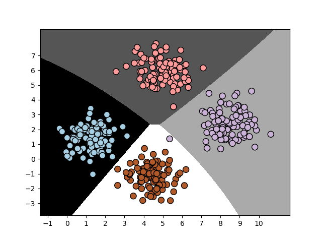
When we run the program we get the following output and graph:

Accuracy of Naïve Bayes classifier = 99.75 %

As usual or program starts with the necessary imports. Then we define the Input file containing data this file is data_multivar_nb.txt is used as the source of data. You can replace this with your own data source file. This file contains comma separated values in each line. Next we load the data from this file.

The we create an instance of the Naïve Bayes classifier. We used the Gaussian Naïve Bayes classifier here. In this type of classifier, we assume that the values associated in each class follow a Gaussian distribution. Next we train the classifier using the training data and then run the classifier on the training data and predicted the output.

We then computed the accuracy of the classifier by comparing the predicted values with the true labels, and then visualize the performance as shown in the graph.

The preceding method to compute the accuracy of the classifier is not very robust. We need to perform cross validation, so that we don't use the same training data when we are testing it. Split the data into training and testing subsets. As specified by the test_size parameter in the line below, we will allocate 80% for training and the remaining 20% for testing. We'll then train a Naïve Bayes classifier on this data. See the code below:

# Split data into training and test data
X_train, X_test, y_train, y_test = train_test_split(X, y,
test_size=0.2, random_state=3)
classifier_new = GaussianNB()
classifier_new.fit(X_train, y_train)
y_test_pred = classifier_new.predict(X_test)

Now compute the accuracy of the classifier and visualize the performance. See the code below:

# compute accuracy of the classifier
accuracy = 100.0 * (y_test == y_test_pred).sum() / X_test.shape[0]
print("Accuracy of the new classifier =", round(accuracy, 2), "%")
# Visualize the performance of the classifier
visualize_classifier(classifier_new, X_test, y_test)

We'll use the inbuilt functions to calculate the accuracy, precision, and recall values based on threefold cross validation. See the code below:

num_folds = 3
accuracy_values = cross_val_score(classifier,
X, y, scoring='accuracy', cv=num_folds)
print("Accuracy: " + str(round(100*accuracy_values.mean(), 2)) + "%")
precision_values = cross_val_score(classifier,
X, y, scoring='precision_weighted', cv=num_folds)
print("Precision: " + str(round(100*precision_values.mean(), 2)) + "%")
recall_values = cross_val_score(classifier,
X, y, scoring='recall_weighted', cv=num_folds)
print("Recall: " + str(round(100*recall_values.mean(), 2)) + "%")
f1_values = cross_val_score(classifier,
X, y, scoring='f1_weighted', cv=num_folds)
print("F1: " + str(round(100*f1_values.mean(), 2)) + "%")


Now when we run the program we get the following output and graph:

The preceding output shows the boundaries obtained from the classifier. We can see that they separate the 4 clusters well and create regions with boundaries based on the distribution of the input datapoints. You will see in the following on terminal and graph as output, the second training run with cross validation:

Accuracy of Naïve Bayes classifier = 99.75 %
Accuracy of the new classifier = 100.0 %
Accuracy: 99.75%
Precision: 99.76%
Recall: 99.75%
F1: 99.75%
------------------
(program exited with code: 0)

Press any key to continue . . .

Read More